Understanding compression of convolutional neural nets: part 3

This is the final post of a three-part series on compressing convolutional neural networks. As indicated in the previous blogs of this series, sometimes you have a resource crunch and you need to reduce the number of parameters of a trained neural network via compression to work with available resources.

In my earlier blog post on this topic, I had shown how to reduce the number of connection weights of a fully connected layer of a convolutional neural network (CNN). In this post, I am going to illustrate how to reduce the number of parameters of a trained convolution layer. The way to do this is to use tensor decomposition which you can view as a technique analogous to matrix decomposition used for fully connected layer compression.

For a detailed introduction on tensors and decomposition, please refer to my three-part series on this topic. Herein, I will only provide a brief introduction to tensors and their decomposition to show how tensor decomposition can be used to reduce the number of parameters in a trained convolution layer.

A brief Tensor refresher

A tensor is a multidimensional or N-way array. The array dimensionality, the value of N, specifies the tensor order or the number of tensor modes. We access the elements of a real-valued tensor

of order K using K indices as in

. Thus, a color image is a tensor of order three or with three modes. Before proceeding any further, let’s look at the following code wherein we use outer product of three vectors to generate a rank 1 tensor.

The above code produces the following tensor of order three:

Analogous to a color image, this tensor has three planes or slices. Now if we have another set of three vectors and perform the outer product calculations, we will end up with another rank 1 tensor of order three. We can then add these two tensors to generate another tensor of order three.

This tensor will be rank 2 tensor because it was generated via combining two rank 1 tensors. Of course, we need not limit ourselves to outer products of triplets of vectors. We can use outer products of quadruplets of vectors to create rank 1 tensors of order four and by mixing r such tensors, we can get tensors of rank r and order k and so on.

Let's now think of the reverse problem. Suppose we have a tensor of order k. Is it then possible to obtain rank 1 tensors whose summation corresponds to the given tensor? Dealing with this problem is what we do in the tensor decomposition method known as CANDECOMP/PARAFAC decomposition, or simply the CP decomposition.

The CP decomposition

The CP decomposition factorizes a tensor into a linear combination of rank one tensors. Thus, a tensor of order 3 can be decomposed as a sum of R rank one tensors as

where (o) represents the outer product. This is illustrated in the figure below.

The CP decomposition is sometimes expressed in the form of factor matrices where the vectors from the rank one tensor components are combined to form factor matrices. For the decomposition expression shown above, the three factor matrices A, B, and C will be formed as shown below:

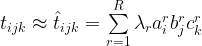
Often, the vectors in rank one tensors are normalized to unit length. In such cases, the CP decomposition is expressed as

where λr is a scalar accounting for normalization. With such a decomposition, a tensor element

can be approximated as

The decomposition is performed by a minimization algorithm, known as alternating least squares (ALS). The basic gist of this algorithm is to keep certain components of the solution fixed while finding the remaining components and then iterating the procedure by switching the components to be kept fixed.

Convolution layer compression using CP decomposition

Now, let’s see how we can compress a convolution layer using the tensor decomposition described above. We will do so by working with a convolution layer specified as Conv2d(3, 2, kernel_size=(5, 5), bias = False). This layer has three inputs and two outputs. Corresponding to each output channel, there is a three-dimensional matrix of 5×5 weights. In our example, we will take the following tensor as the weight tensor of our convolution layer.

Let’s represent the input tensor as X(i, j, k) and the corresponding output as Y(m, n, p). We can relate the output with the input through the following expression where W(i, j, k, p) is the 5x5x3x2 weight tensor:

After performing tensor decomposition with R rank 1 components, you can write the output as

,

where

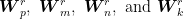
are four-factor matrices of size 2xR, 5xR, 5xR, and 3xR, respectively. Note the dimensions of these factor matrices. These are tied to the number of input and output channels, convolution mask size, and of course the rank of the approximated tensor.

Since we have R rank 1 components, we need input channels to merge to R parallel paths to perform convolution and then merge these paths to generate the number of specified output channels.  This suggests the following sequence of steps using the factored matrices to perform convolution in four stages.

1. Perform 1×1 convolution using the factor matrix

. In our example, this will map three input channels to R channels.

1. Perform in parallel, convolutions using the factor matrix

.

1. Continue with convolutions using the factor matrix

. The convolutions in steps 2 and 3 are separable convolutions and together result in convolution in both horizontal and vertical directions.

1. Combine the result of Step 3 via 1×1 convolutions to produce the required number of output channels.

Now, let’s apply the above decomposition steps to our example layer. We will perform the tensor decomposition using python library Tensorly.

Thus, we have the factor matrices for implementing the convolution layer through the four steps mentioned above. Let’s look at the factor matrices obtained via the CP decomposition. Tensorly gives the following output for factors:

Let’s designate the factor matrices as:

Now we can implement the convolution layer through the above factor matrices as shown below. Note the use of groups parameter to perform convolutions in parallel.

Now it's the time to see how well the convolution layer approximation by the CP decomposition performed. We will do so by creating an arbitrary input tensor. I used the following tensor as an input.

Using the above tensor as input, I calculated the output first by the convolution layer without any approximation, and then by the approximate implementation. The norm of the difference between two outputs was then calculated and expressed as a percentage of the output without any approximation. This came out as 26.2571%. A rather large number. To understand why the error is so large, I decided to look at the approximated tensor. You can get the approximated tensor by carrying out the outer products between the components of every rank 1 tensor and then adding them as we did at the very beginning of this post to create a tensor. Tensorly also has a function to do this.

You can see that the approximated tensor is much different from the original tensor. This is because R being equal to 2 is not sufficient and may be R needs to go higher. Anyway, to get an idea of the tensor approximation error, I calculated the norm of the difference between the original tensor values and those of the approximated tensor. After normalizing it, this error turns out to be 35.6822%. Thus, the error in the convolution output because of approximation is in line with the approximation being performed in tensor decomposition.

You might be wondering about the amount of decompression achieved in this example. We had 150 weight values defining the convolution masks in the original implementation. With decomposition, the number of factored matrices elements is 30. Thus we are able to achieve 80% reduction. Of course, the approximation is too crude. Assuming that R equal to 3 will yield an acceptable approximation, we will then be needing 45 values to define different mask elements; it is still a significant reduction.

As an example of decompression that can be achieved in a real network, let’s look at  the first convolution layer of the VGG-19 network. The layer is defined as Conv2d(3, 64, kernel_size=(3, 3), stride=(1, 1), padding=(1, 1)). Thus, the layer has 64 output channels, 3 input channels, and the convolution masks are of size 3×3. The layer weight size is thus [64, 3, 3, 3], meaning we need 1728 values to specify the masks. It turns out that R equal to 16 yields a fairly good approximation. In that case, the factor matrices are of the (64, 16), (3,16), (3,16), and (3,16).

The total number of elements in these matrices is 1168, about 2/3rd of the elements without decomposition. In practice, a suitable value for R has to be figured out to optimize decompression ratio while keeping the approximation at the accepted level.

Before wrapping up this post, let me mention that there is another decomposition method, known as the Tucker decomposition. It is extremely efficient in terms of approximation and allows different number of components in different modes which is not possible in CP decomposition. Similar steps can be followed to reformulate convolution layers using the Tucker decomposition. For those interested in seeing how the Tucker decomposition will be applied, I highly recommend visiting this site.