
This is second part of a three-part series of blog posts about compression of deep neural networks. The compression, which reduces the number of parameters and computation, is a useful technique for deploying neural networks in environments such as in edge computing where compute power, memory space, battery power, etc. are limited. In such instances, compressing neural networks before deployment allows greater use of available resources.
In the first part of the series, I had explained the matrix factorization technique, singular value decomposition (SVD), which is the basis of compression methods. In this post, I will show how to perform compression of feedforward neural networks using SVD. The compression of convolutional networks will be covered in the next post.
Feedforward neural network
A feedforward neural network consists of an input layer, one or more hidden layers, and an output layer. The input layer size equals the number of features being used. The number of hidden layers and their size is a choice made by the network designer. Theoretically, one hidden layer is all that is required to learn any input-output mapping by the network. The output layer size depends upon the number of classes for classification problems. For regression, only one output neuron is needed.
A trained neural network operates only in the forward mode of computation. For a network with m inputs, n (n < m) neurons in the hidden layer, and p output neurons as shown below, the forward computation can be defined through the following relationships:
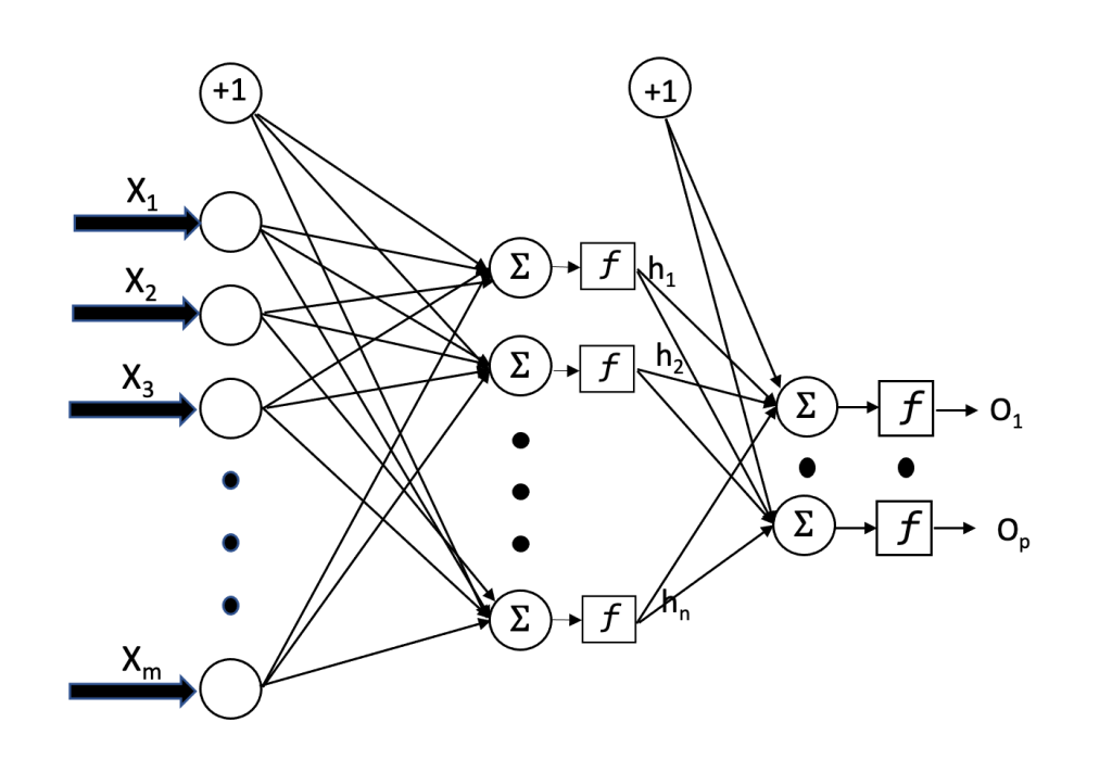
Let WI be the m x n weight matrix representing the connection weights for links between the input layer and the hidden layer. Let b be a vector of size n x 1 representing the bias weights to hidden layer neurons. The linear summation computed by hidden layer can be then expressed as

Let h be a vector of size n x 1 representing the output of the hidden layer after passing the linear summation through a non-linear activation function f. We then have

Let’s absorb b after transposing it as a row vector into the weight matrix and represent the augmented weight matrix as W with m+1 rows and n columns. Let’s also augment the input vector X by adding 1 at the end of the vector. With that, the hidden layer output can be expressed as

Following the similar steps, the output vector o of size p x 1 can be expressed as

,
where Z is the augmented matrix representing the link weights from the hidden layer and the bias weights to the output layer.
Compressing a feedforward neural network
Looking at the forward computation performed by a trained feedforward network, we see that there are two matrices, W and Z that can be subjected to singular value decomposition to achieve compression. We will just consider the decomposition of W for illustration. Through SVD, we can express W

,
where U is of size (m+1) x n, V is of size n x n, and the matrix D is of size m x n with singular values as its diagonal elements. An approximation of the augmented weight matrix using only top r singular values is given as

,
Let’s use this approximation in the forward computation expression to re-write the hidden layer output as

The above expression can be expressed as

Through matrix transpose, we can further write the above expression as

Looking at the above expression, we see that the forward computation to calculate the hidden layer output can be carried out as follows:
- First, calculate the intermediate output

. This involves only (m+1) x r weights.
- Next, use the intermediate output to multiply it with

This involves only r x n weights.
- Use the output of Step 2 to pass it through nonlinearity to get the hidden layer output.
We can see that the decomposition of the weight matrix reduces the number of weights to (m+n+1) x r as opposed to the number of weights, (m+1) x n without decomposition. With r << n, we can see a significant compression in the number of weights (parameters) as well as in multiplications.
Let’s apply compression to a trained network for illustration purposes. We will do so by working with the Wine data set; this data set consists of 178 observations from three classes of wine and each observation consists of 13 features. We will use the Scikit-learn library for training with the feedforward network consisting of a single hidden layer of 10 neurons. As you look at the code, remember the input vectors are represented as row vectors.
import numpy as npfrom sklearn.neural_network import MLPClassifierfrom sklearn.model_selection import train_test_splitfrom sklearn.preprocessing import StandardScalerfrom sklearn.datasets import load_winefeatures, target = load_wine(return_X_y=True)X_train, X_test, y_train, y_test = train_test_split(features, target, test_size=0.30, random_state=15)scalar = StandardScaler()scalar.fit(X_train)X_train_scaled=scalar.transform(X_train)X_test_scaled = scalar.transform(X_test)mlp = MLPClassifier(hidden_layer_sizes =10,activation = 'tanh', learning_rate_init=0.01,batch_size=10,solver='lbfgs', random_state=0).fit(X_train_scaled, y_train)result = mlp.predict(X_test_scaled)print("Training_accuracy: {:.2f}".format(mlp.score(X_train_scaled, y_train)))y_pred = mlp.predict(X_test_scaled)print("Test_accuracy: {:.2f}".format(mlp.score(X_test_scaled, y_test)))y_pred = mlp.predict(X_test_scaled) |
Training_accuracy: 1.00 Test_accuracy: 0.96
Let’s now look at the connections weights between the input layer and the hidden layer. We also need to look at the bias weights.
W = mlp.coefs_[0]b = mlp.intercepts_[0]print(W.shape)print(b.shape) |
(13, 10) (10,)
We see that the weight matrix is of size 13×10 and the bias weights are represented as a column vector of 10 values. In order to perform compression, let’s first combine the connection weight matrix and the bias weights into a single matrix.
W_i = np.concatenate((W, b.reshape(1,-1)),0)print(W_i) |
[[ 0.666 0.425 -0.669 0.704 -0.844 0.141 0.262 0.058 0.427 -0.901] [ 0.314 -0.135 -0.016 0.04 -0.445 -0.546 -0.369 0.109 0.124 0.154] [ 0.551 0.347 -0.367 0.686 -0.445 0.006 -0.308 0.312 0.012 -0.667] [-1.181 -0.014 0.684 -0.463 0.202 -0.288 -0.273 0.538 0.145 0.697] [-0.011 -0.109 -0.024 -0.237 -0.136 0.331 -0.362 -0.62 -0.192 -0.297] [ 0.402 0.054 0.368 0.115 -0.262 -0.047 0.216 -0.489 0.309 -0.269] [ 0.014 -0.727 0.14 -0.844 -0.025 0.356 0.443 -0.83 0.966 0.181] [ 0.231 -0.061 0.482 -0.224 0.457 -0.42 -0.279 -0.071 -0.433 0.068] [-0.203 -0.149 -0.286 -0.038 0.528 -0.216 -0.078 -0.158 0.121 0.514] [-0.074 0.55 -0.72 0.872 -0.562 -0.576 0.217 -0.12 -0.207 -0.96 ] [-0.038 -0.535 0.453 -0.191 0.077 0.497 -0.015 -0.163 0.176 1.157] [ 0.474 0.194 0.01 -0.244 0.095 0.252 0.468 -0.408 0.942 0.031] [ 1.103 0.253 -0.389 1.109 -0.883 0.312 -0.206 -0.66 0.439 -1.219] [-0.242 -0.374 -0.278 0. -0.106 0.32 0.104 -0.048 0.183 -0.251]]
Now we are ready to perform the decomposition of the augmented weight matrix.
from scipy import linalgU,s,Vt = linalg.svd(W_i)print(U.shape,Vt.shape)print('Singular values \n',s) |
(14, 14) (10, 10) Singular values [3.991 2.462 1.356 1.172 1.076 1.009 0.856 0.687 0.59 0.415]
As expected, the size of the U matrix is 14 x 14 and of V matrix is 10 x 10. Out of 10 singular values, the top two values are relatively much higher than the rest of the values. Based on this observation, let us decompose the augmented weight matrix using only the top two singular values. The decomposed matrices are formed as follows.
diag = np.array([[s[0],0],[0,s[1]]])U_2 = U[:,0:2]Vt_2 = diag@Vt[0:2,:] |
Using these decomposed matrices, we will now check the performance of the network on the test data. This will tell us whether any degradation in the accuracy occurs or not.
test_aug = np.append(X_test_scaled, np.ones(len(X_test_scaled)).reshape(-1,1),1)test_int = test_aug@U_2 # Calculate the intermediate resulttest_hin = test_int@Vt_2 # Result is the linear sum at hidden unitstest_hout = np.tanh(test_hin)# add a column of 1's to account for biashout = np.append(test_hout, np.ones(len(test_hout)).reshape(-1,1),1)Z = np.concatenate((mlp.coefs_[1],mlp.intercepts_[1].reshape(1,-1)),0)test_out = hout@Z # output of the network for test vectorsaccuracy = 1-np.sum(result!=y_test)/len(X_test_scaled)print('The test accuracy with compression is = ', accuracy) |
The test accuracy with compression is = 0.962962962962963
We see that the accuracy after compressing the first layer is not impacted. The number of weights in the first layer without compression is 14 x 10 but with compression we only need 14 x 2 + 2 X 10, that is 48 weights. This gives us about 2/3 compression of number of weight values. Including the output layer weights, the compressed network requires 81 weight values. Obviously, this simple example while illustrating the compression may not strongly justify it. But when you think of fully connected layer in deep convolutional networks with 1000 categories at the output and millions of weights, the advantage of compression becomes obvious.
Compression using Truncated SVD
The decompression carried out above only changed the way the hidden layer output was calculated. When performing compression using truncated SVD, the weight matrix is not only approximated but its size is changed as well. This change in size modifies the number of hidden layer neurons also. This means that the Z matrix of the trained network cannot be used and the hidden-layer to output layer weights must be obtained by another training round. An important consequence of this is that the training data must be available for re-training the output layer.
I will now illustrate the compression using the truncated SVD using the neural network used above. In the code given below for this, I will first get the reduced matrix for the first layer; use this reduced matrix to calculate the reduced hidden layer output for the training examples. This output will be then used to train the output layer.
from sklearn.decomposition import TruncatedSVDdim_red = TruncatedSVD(2, algorithm = 'arpack')Wr = dim_red.fit_transform(W_i)train_in= np.append(X_train_scaled, np.ones(len(X_train_scaled)).reshape(-1,1),1)hout = np.tanh(train_in@Xr)# Output of new hidden layerhout = np.append(hout, np.ones(len(hout)).reshape(-1,1),1)#Now we train last layer with hout as input.from sklearn.linear_model import LogisticRegressionclf = LogisticRegression(random_state=0).fit(hout, y_train)test_in = np.append(X_test_scaled, np.ones(len(X_test)).reshape(-1,1),1)train_acc = clf.score(hout,y_train)test_acc = clf.score(np.tanh(test@Xr),y_test)print('Train Accuracy = ', train_acc)print('Test Accuracy = ', test_acc) |
Train Accuracy = 0.9838709677419355 Test Accuracy = 0.8888888888888888
So in this, the train and test accuracy go down as a result of decompression. This should not be surprising as the number of hidden layer neurons went down to 2 from 10. The number of weights in the compressed network is only 34 (14 X 2 + 3 X 3), compared to 177 (14 X 10 + 11 X 3) of the original network, a significant reduction, and compared to 81 weights of the network compressed with SVD.
To summarize, the SVD based compression of neural networks offers a way of optimizing resources in constrained environments with a potential minor loss in the network accuracy. The truncated SVD can offer much more compression but it comes with a higher performance loss and thus must be used with care. In the next post, we are going to look at compression of convolutional layers of deep neural networks.


AI accelerator insider insider
Thank you for subscribing
Level up your ai accelerator insider career & network with ai accelerator insider experts.
An email has been successfully sent to confirm your subscription.
 Follow us on LinkedIn

