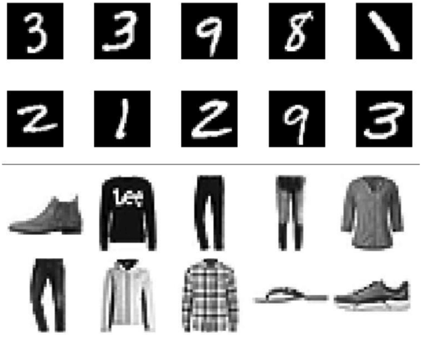
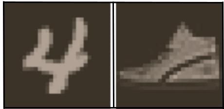
I want you to take a minute and try to read out the numbers in the picture above. Then, call out the clothing items that you see below these numbers. Easy, right? Well, what if I told you this was a challenging task for some people, and by some people I mean...my computer.
Wait, what…a computer? Yes! Just recently, when diving into what is now my deepest passion, Artificial Intelligence, I realized that machines, like computers, could classify all sorts of images. Due to my curiosity, I wanted to make two feedforward neural network models: one that could classify numbers and another that could classify clothing items!
In this article, you'll have insight into:
Let’s backtrack for a minute…what’s a feedforward neural network?
Encompassed in Artificial Intelligence (AI) is a subsection that consists of neural networks. Neural networks are essentially made up of artificial neurons or nodes that form connected layers.
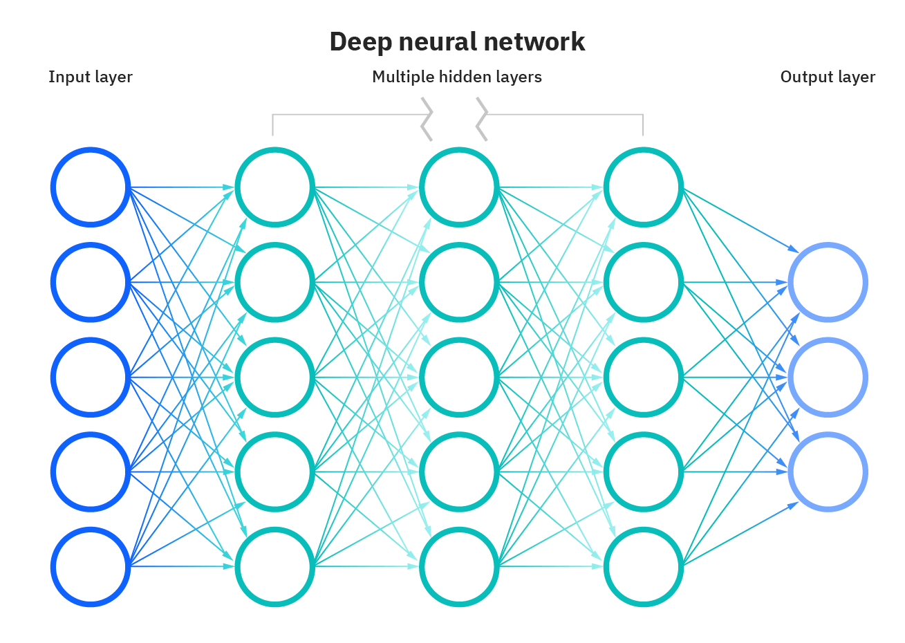
Typically, a neural network has a similar architecture as the picture above. It starts off with an input layer that takes in certain data from a specific dataset and ends off with an output layer that predicts the final outcome. In between, there are hidden layers that perform complex computations in the network to get from the input to the output layer. If there is more than one hidden layer, then the neural network is “deep”.
Connecting the nodes
My projects consist of deep feedforward neural networks, which means that the network only moves in one direction: forward, from the input layer to the many hidden layers to the output layer. Furthermore, it resets after every epoch, which is one complete run through all of the data forwards and backward when training/testing, making the accuracy higher.
The projects’ datasets
Before I walk you through my code in small increments, let me give you a bit of background information about the datasets to make it easier to understand some complex syntax that is performed with these datasets.
The images of the numbers and clothing items both come from a torchvision package from PyTorch, which is the programming framework I used to compute the neural network model. In the torchvision package, there are MNIST datasets. So, for one model, I used the Number MNIST dataset and the Fashion MNIST dataset for the other.
These datasets each contain 60,000 small squares of 28 by 28 pixel images. The Number MNIST dataset contains handwritten 1-digit numbers (0–9) and the model outputs one of these numbers. The Fashion MNIST dataset is similar because it contains 10 classes/choices of outputs, but the data is of clothing items, like a sandal, t-shirt, coat, etc. Despite the data being clothing items, the labels are in the form of numbers 0–9.

Please note: the code of these feedforward neural networks is very similar, except for some tiny changes. I will point out these out in the next couple of sections.
The code I’m explaining is in small chunks. However, if you’d like to see what my whole project looks like and use/refer to it, check out my Github repository for these 2 projects.
Without further ado, let’s dive deep into the code, which is split up into 6 crucial parts:
- Importing Libraries
- Importing the Datasets and Splitting up the Training and Testing data
- Building the Neural Network Model
- Training the Model
- Testing the Model
- Visualization
Step 1: importing libraries
import torch
from torch import nn
from torch import optim
from torchvision import datasets, transforms
import helper
In this step, we import essential libraries that will be used in further steps:
torch— we need this library and numerous packages included in it, includingnnandoptim, since they are crucial for the next steps in the process.- We also imported
datasetsandtransformsfromtorchvision, which as I mentioned, contains the data we need to input for the model. - The
helperandmatplotlib.pyplotlibraries are used to show data and graphs to describe features the model has, such as its training loss (we will get into this later).
- Note that the first line in the code above means that the output of the matplotlib plotting commands will be displayed inline, right below the running code cell in a Jupyter notebook (as shown to the right).
Step 2: importing the datasets and splitting up the training and testing data
transforms.Normalize((0.5,), (0.5,))])
This piece of code defines a variable to transform the images by making them more suitable, which is necessary for later computations.
- The
ToTensor()function converts a pixel that has a range from 0 to 255 to a pixel range of 0 to 1. - The
Normalize()function has 2 parameters and, in this instance, the first parameter and the second parameter are both contain (0.5,). If later on, the normalize attribute is true when applied to a set of images, the images will be grey-scaled.
After defining this variable, you need to get the data from the MNIST datasets in torchvision:
trainloader = torch.utils.data.DataLoader(trainset, batch_size=64, shuffle=True)testset = datasets.MNIST('~/.pytorch/MNIST_data/', download=True, train=False, transform=transform)
testloader = torch.utils.data.DataLoader(testset, batch_size=64, shuffle=True)
In the code above, we have 2 similar segments: one for the training data and one for the testing (synonymous to evaluation or validation) data, which downloads and loads the necessary data.
- There are 2 variables for downloading the datasets:
trainsetandtestset. Both the training and testing sets contain similar arguments, including the path from the dataset to the MNIST data, whether the dataset should be downloaded (set toTrue), and the transformations from thetransformvariable that need to convert the image data. However, in the train set, the train argument is set toTruebecause that data is going to be used for training, which is a different case in the test set. - There are also 2 variables following the trainset and testset, respectively. These data loaders load these datasets, change their batch size (the number of samples that passed through to the network at one time), and shuffle the data is after every epoch.
Note: the Fashion MNIST dataset follows the same syntax as shown above, but the path to the dataset is "~pytorch/F_MNIST_data/" instead.
To ensure that the data has downloaded and loaded properly, we can run this:
helper.imshow(images[0], normalize=True)
This would end up giving us an arbitrary image (images[0]) in the training dataset that is grey-scaled, since normalize=True.
Step 3: building the neural network model
hidden_layers = [256, 128, 64]
output_layer = 10model = nn.Sequential(nn.Linear(input_layer, hidden_layers[0]),
nn.ReLU(),
nn.Dropout(p=0.2),
nn.Linear(hidden_layers[0], hidden_layers[1]),
nn.ReLU(),
nn.Dropout(p=0.2),
nn.Linear(hidden_layers[1], hidden_layers[2]),
nn.ReLU(),
nn.Dropout(p=0.2),
nn.Linear(hidden_layers[2], output_layer),
nn.Softmax(dim=1))
This part of the code is fairly straightforward if you understand the neural network architecture. When coming up with the model, there are three necessary questions to consider:
- How many layers are there?
- How many nodes are there in each of those layers?
- What transfer/activation function is used in each of those layers?
This code initializes variables relating to the number of nodes in each layer and then adds different features to it, like the activation and dropout functions.
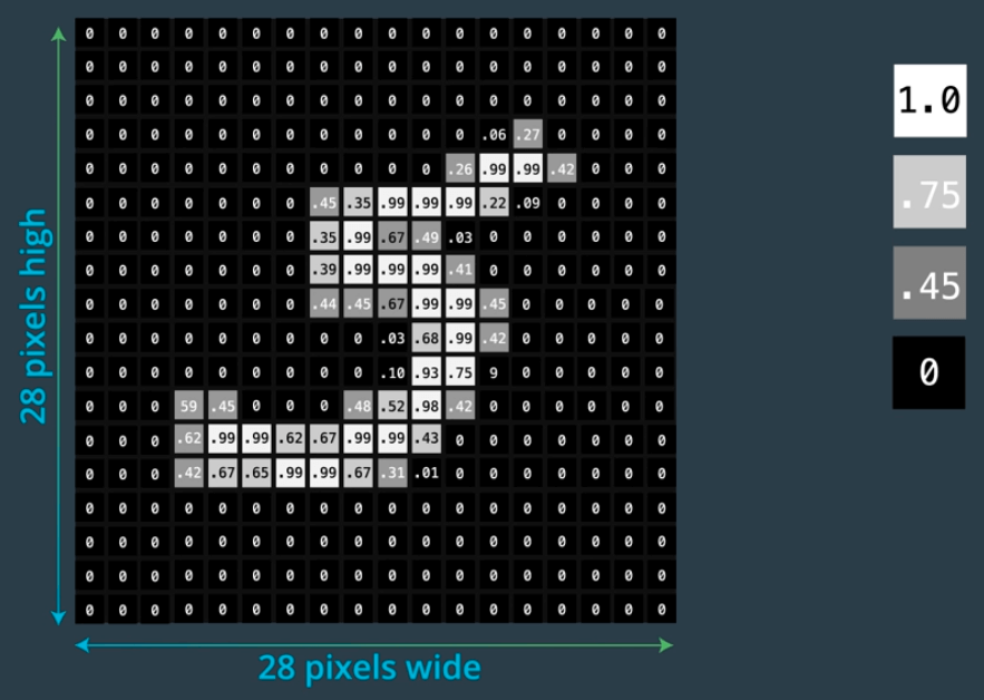
- There are 784 nodes in the input layer because when changing the 28x28 pixel image into a 1D vector, it would have a length of 784. This makes sense because you want to input 1 pixel into one node and compute based on that.
- The hidden layers can be arbitrary numbers between the number of input and ouput layer nodes, but the output layer has to be 10 because there are ten possible outcomes from the neural network model.
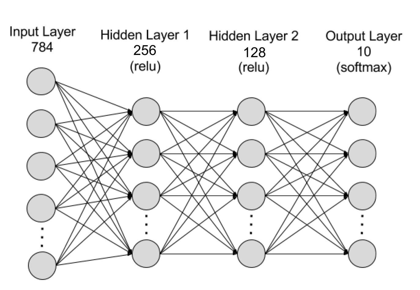
As the picture above portrays, the model needs the ReLU and Softmax functions, which acts as activation functions in the neural network, and the Dropout function to prevent overfitting (when the model is too aligned with the training data, hence does poorly on the testing data).
Note: the Fashion MNIST model has 3 hidden layers [256, 128, 64] because they’re used to increase the model’s accuracy later on.
Step 4: training the model
To easily conceptualize the training process, think of training the model as trying to shoot a 3-pointer for the first time (you obviously won’t be like Steph Curry and get it in every time 😉). Also, to measure how far off you were from getting it in, you use the shortest distance between the net and the ball → called the loss. You’d probably air ball the first time and realize that the loss was large. Then, you change your technique, strive for a lower loss, and continue this cycle again and again until you get fairly decent accuracy.
This is analogous to what happens when a neural network model is being trained:
total_training_loss = 0
for images, labels in trainloader:
images = images.view(images.shape[0], -1) optimizer.zero_grad()
logps = model(images)
loss = criterion(logps, labels)
loss.backward()
optimizer.step()total_training_loss += loss.item()
In the code above, specifically:
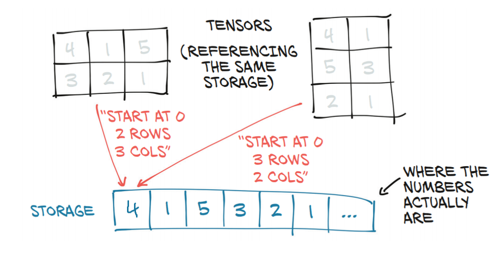
- The images and their labels are taken from the training dataset. The images are flattened because they’re currently 2D tensors but need to be 1D vectors. In this instance, takes the size of the images, which is
1 x 28 x 28 and keeps theimages.shape[0]which is 1. Then, it merges the remaining dimensions into one number, figuring out an appropriate size(784 → 28 x 28). This way, the model adjusted itself from 1 x 28 x 28 (2D tensors) to 1 x 74 (1D vector). - Then, you use the
optimizer.zero_grad()to set the gradients of the model to 0. The gradients are the change in all weights (values that control the strength of the connection between two neurons) with regards to the change in error/slope. Clearing the gradients from each prior epoch is needed, so the results don’t “collide”🚗 with each other and cause hard-to-deal-with errors 😂. - The
logpsruns all the images into the model we defined earlier. - The
criterion = nn.NLLLoss()function is defined outside the “for” loop and uses nn module’s “Negative Log-Likelihood Loss”. This is later used in thelossvariable, which finds the difference between what the image shows and what the label says. Since the criterion uses NLLLoss, the loss will always be negative and the closer it gets to -1, the more accurate it is. At the end of step 4, the total loss of entire mini-batch divided by the batch size is added to the total training loss. - The next part of this step is to use the
backward()function and apply it to the loss, which runs through the model backwards (back propagation). - Furthermore, we use
optimizer.step()to update the weights when doing a backwards pass through the model → called gradient descent.
Step 5: testing the model
Now that we have trained our model, we need to actually test this model out to understand how the model does with unseen data. The training and testing code blocks are fairly similar, but the testing requires more syntax to print out the results of the epoch it’s currently running through, the losses, and the accuracy of the model when testing.
total_testing_loss = 0
test_correct = 0
with torch.no_grad():
model.eval()
for images, labels in testloader:
images = images.view(images.shape[0], -1)
logps = model(images)
loss = criterion(logps, labels) total_testing_loss += loss.item() ps = torch.exp(model(images))
top_p, top_class = ps.topk(1, dim=1) equals = top_class == labels.view(*top_class.shape) test_correct+=torch.mean(equals.type(torch.FloatTensor))
model.train()
When testing the model, we need to have two important variables: the total_testing_loss and the amount of times the model classifies the image correctly within the testing dataset (used to determine the accuracy).
- Since this piece of code is for testing, it doesn’t need to adjust the gradients, so we use
torch.no_grad()to turn it off. - It also doesn’t need dropout when testing, so we use
model.eval()to turn dropout off and then turn it back on after testing. As a result, when going back to the top of the loop for the next epoch, it uses dropout for the training again. - The next few lines are analogous with the training data loop since they take the images and labels from
testloader, view them as a 1D vector, find the loss, and add it to thetotal_testing_loss. - The ps variable gets the probabilities of the images being each class. Then,
ps.topk(1, dim=1), which contains the highest class probability of each image is split into two: the highest probability of the images(top_p) and the classes associated with them(top_class). - Next, the equal variable is either set to True or False. It will be True (1) if the predicted class and the label are the same or False (0) if they aren’t. All the numbers will be added and the mean will be calculation and added to
total_correct.
test_losses.append(total_testing_loss / len(testloader))print("Epoch: {}/{}.. ".format(e+1, epochs),
"Train Loss: {:.3f}.. ".format(train_losses[-1]),
"Test Loss: {:.3f}.. ".format(test_losses[-1]),
"Test Accuracy: {:.3f}".format(test_correct/len(testloader)))
After evaluating the model, right under model.train() from the previous code block, the average training loss and testing loss are calculated for that certain epoch. Lastly, the current epoch, training loss, testing loss, and accuracy are printed in a decimal format going up to 3 decimal places.
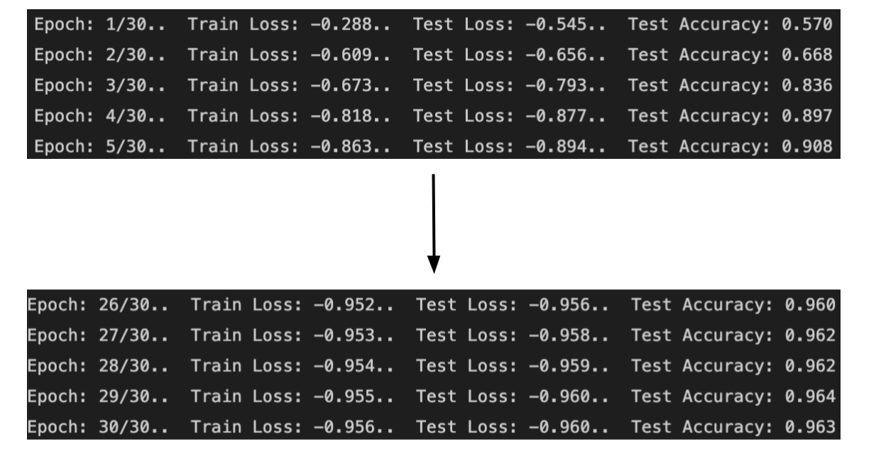
The above is what is printed after 30 epochs. Here, the training loss and the testing loss get closer and closer to 0, while the test accuracy gets closer and closer to one. As it turns out, just as if you were to practice shooting three pointers 🏀 repeatedly, the accuracy would increase. Here, the accuracy went from 57% TO 96%.
Note: for the Fashion MNIST model, the accuracy went from 21% to 82%. The accuracy is lower than the Number MNIST model because the images are more complex and would be classified better with CNNs, which is an image classification neural network that I’ll be diving deep into in the coming weeks.
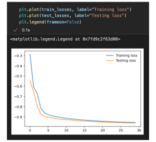
To help comprehend these numbers, we can put them into a simple graph using matplotlib.pyplot as plt.
plt.plot(test_losses, label=”Validation loss”)
plt.legend(frameon=False)
The above code prints out this double-line graph comparing the training loss and testing loss.
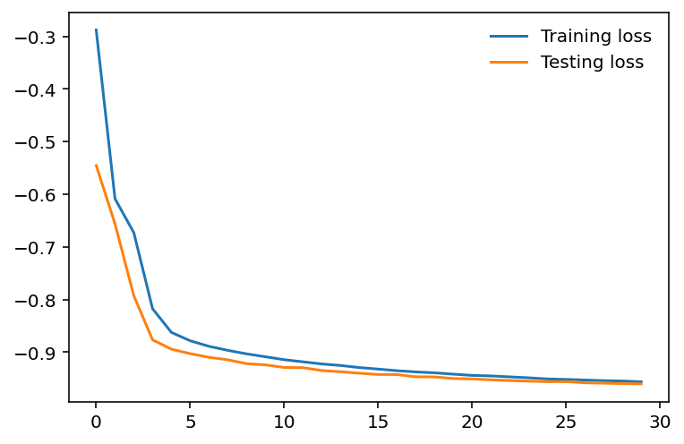
- With
plt.plot(), we graphed a line for the training losses and the testing losses with regards to the number of epochs. - Then, the
plt.legend()gives the plot a legend. This legend becomes borderless (won’t have a box around it) when theframeonattribute of that function’s set toFalse.
Step 6: visualization
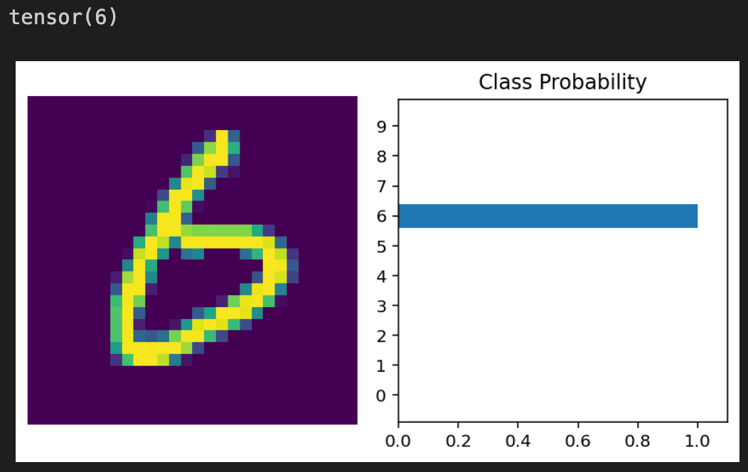
We know our model works due to the low loss and high accuracy we get after training and testing. So, let’s look at an example to visualize what the model outputs:
images.resize_(images.shape[0], 1, 784)ps = model(images[0,:])
helper.view_classify(images[0].view(1,28,28), ps)
print(labels[0])
This code goes through all the images, which to recap, are shuffled after every epoch. It then resizes all the images into a 1D vector.
- The
psvariable puts all the images through the model and gets the probabilities of the image as each class. helper.view_classifydisplays 2 visuals: the first image in the set of images fromtestloaderand a bar graph displayingps. Lastly, to confirm if the model was correct, we print the label corresponding to the first image.
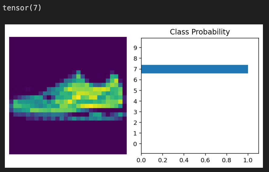
The Fashion MNIST model has the same code when it come to visualization, but as expected with the different datasets, they have different outputs.


AI accelerator insider insider
Thank you for subscribing
Level up your ai accelerator insider career & network with ai accelerator insider experts.
An email has been successfully sent to confirm your subscription.
 Follow us on LinkedIn