
I love wearing pink pants during my talks, which has become one of my signature looks. I own multiple pairs, which has sparked many discussions about fashion and style. Recently, I have been involved in a project called "Fashion AI," where we utilize a fine-tuned model to segment clothing in images.
We then crop out each labeled article and resize the images to the same size. Finally, we store the embeddings generated from those images in Milvus, an open-source vector database that can store and query billions of vector embeddings.
To find the closest matching articles in our database, we apply the same transformations to the image and the query along the same vectors. For each query, this project returns three results. You can interpret the results based on your preference. You can also determine which celebrity is the closest match for you. You may choose the most common first place, the lowest aggregated distance, or the most common overall.
You can find the images here. In addition to the images, you will need an upgraded Python version and `pip install milvus pymilvus torch torchvision matplotlib`. We use the clothing segmenter model from Mateusz Dziemian on Hugging Face, and this ResNet50 model from Nvidia on PyTorch for image segmentation and embeddings.
In this post, we’ll discuss how to generate image segmentation for fashion items, add your image data to Milvus, and find out which celebrity your style is most like.
Image segmentation for clothing articles
To perform image segmentation, I have found three models to look at on Hugging Face.
- The segformer_b2_clothes by Mateusz Dziemian
- The YOLOS-Fashionpedia by Valentina Feruere
- The Fashion-CLIP model by Patrick John Chia
I ultimately chose the "segformer" model. It provides accurate segmentation for different articles of clothing and identifies 18 types of "objects." For example, it detects "upper clothes" for any kind of tops, "dress," "left shoe," "right shoe," "hat," and many more articles of clothing. In addition, it can detect things like "face," "hair," "right leg," and "left leg." You can find the full set of 18 object types here.
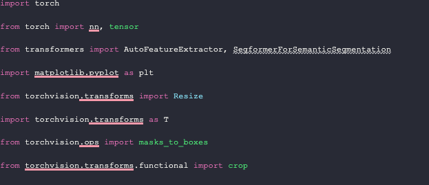
We begin by importing the necessary packages for image manipulation in this project. These include `torch` for feature extraction, `segformer` object from `transformers`, `matplotlib`, and some `torchvision` imports such as `Resize, masks_to_boxes`, and `crop`.
Generate segmentation masks with HuggingFace
There are many approaches to segmenting your image, depending on the model you use and what it detects. For this example, our model returns an 18-layer image, one for each object type, including the background. The first function we need to write is one that generates this image.
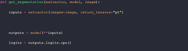
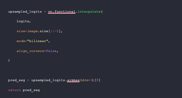
The `get_segmentation` function requires three parameters: a feature extractor, a model, and an image. First, it generates input features using the image and extractor. Then, it obtains the model output and converts it into logits. Afterward, it upsamples the logits through a PyTorch bilinear interpolation. Finally, the function takes only the maximum prediction for each pixel in the upsampled samples to create a segmentation mask.
For reference, the images in `upsampled_logits` look like this:
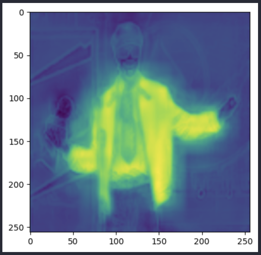
Whereas the `pred_seg` image looks like this: (these are two different images, although both are of Andre 3000)

Getting the segmentation masks is straightforward from here. We obtain all the unique values in the segmentation; in this model, there can only be up to 18. We discard the first entry, which represents the background. To create the masks, we extract the pixels in the segmentation that have the same value as the object ID. I make this function return both the masks and the IDs so that we can keep track of both.
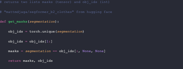
This function creates masks that look like this (hair and upper clothes masks shown):
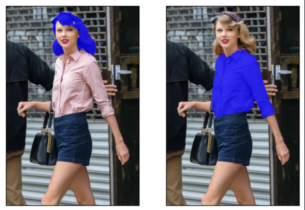
Fameflynet Pictures via Buzzfeed
Crop and resize your images with Pytorch transforms
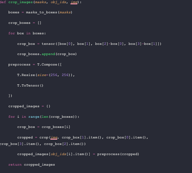
We can now create a new image for each detected object using the `get_masks` function's masks and object ideas, as well as the original image. Then, we call trhe magical `masks_to_boxes` function, which we imported earlier from `torchvision.ops`, to convert the created masks into bounding boxes.
Next, we create a list of boxes to crop and convert the box coordinate system into the `crop` coordinate system. The boxes are returned as values in the form of `(x1, x2, y1, y2)`. On the other hand, the `crop` function expects an input in the form of `(top, left, height, width)`.
Before we crop the images, we also define a preprocessing function. We want to resize each image to 256x256 and convert them into PyTorch Tensors (currently PIL Images). Now it’s time to crop the images. We loop through the crop boxes and call the `crop` function on the image using the values we got earlier. Then we add the preprocessed image as the value corresponding to the key value of the segmentation id to a dictionary. At the end of the function, we return that dictionary.
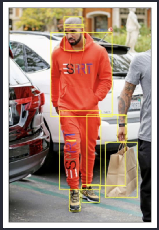
Below is an example of the boxes we crop and create separate images for using Drake in a fire output.
Add your image data to a vector database
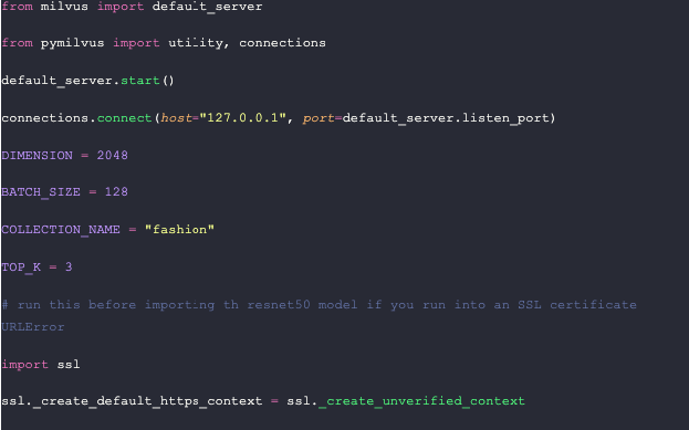
Now that we have all the images segmented and cropped, let’s add them to Milvus, our vector database. To help you get started with Milvus quickly, we use Milvus Lite, a lightweight version of Mivlus, in this example to run an instance of Milvus in our notebook. Then we use `pymilvus` to connect to the default server provided by Milvus Lite.
We also use this section to set up some constants. Let’s define the number of dimensions in a vector (from the Nvidia ResNet50 model), the batch size, the name of our collection, and the number of results to return. Finally, we run an `ssl` function to create an unverified context to get the model from PyTorch.
Defining your schema to store metadata in a vector database
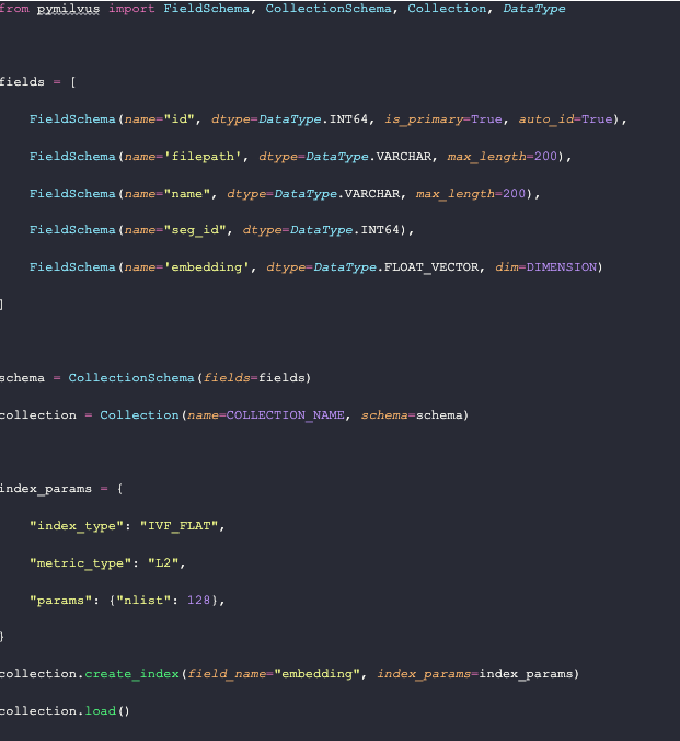
Step one: define your schema. The schema is used to organize the data saved in the vector database. The `id` field is a regular key ID in SQL or NoSQL databases, while the other fields have SQL-like definitions in their data types (int64, varchar, float, etc).
For this example, we save the file path, the celebrity's name, and the segmentation ID as metadata. In the future, we may add more fields, such as the location of bounding boxes or masks. Once we define the FieldSchema, we define a CollectionSchema, and then create a Collection in Milvus based on the given schema and collection name.
Now that we have a collection, let's define its index. These index parameters are pretty basic. We use IVF Flat with 128 centroids and L2 as the distance metric. We create the index in our collection, specifying that the `embedding` field is the one to operate on. Then, we load the collection into memory so that it is ready to be operated on.
Getting your vector embeddings from Nvidia’s ResNet50
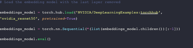
The first step in this section is to load the model. We load Nvidia’s ResNet50 model from PyTorch, then we cut off the output layer. Vector embeddings are the output of the second to last layer in a model.
This function is responsible for receiving the vector embeddings and inserting the data into Milvus. It accepts three parameters: the data, the collection object, and a model, which in this case is the embedding model. To keep track of how the data is being operated as we add it to our vector database, I have added several print statements.
In addition to printing debugging data, we stack all the values in `data[0]` into one tensor and then remove any dimensions of size 1 from the output using the `squeeze` function. Then, we insert a new list consisting of the last three entries of the original data batch, followed by the output tensor converted into a list. These correspond to the file path, name, segmentation ID, and the 2048 dimensional embedding.
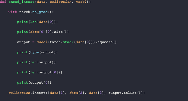
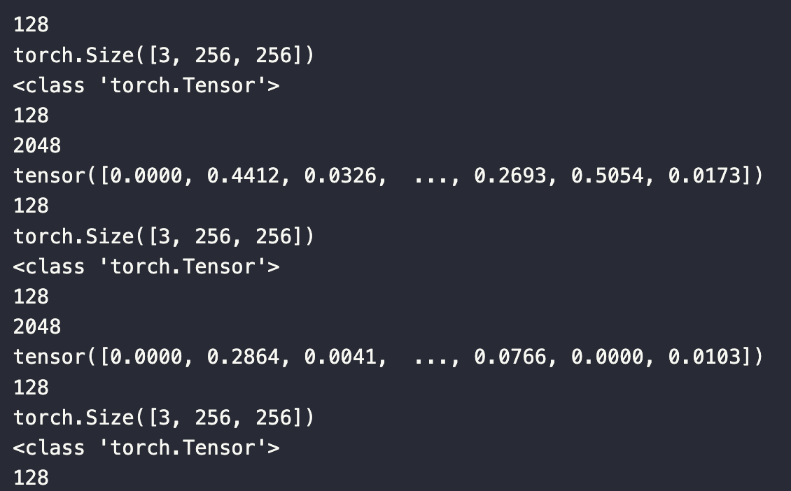
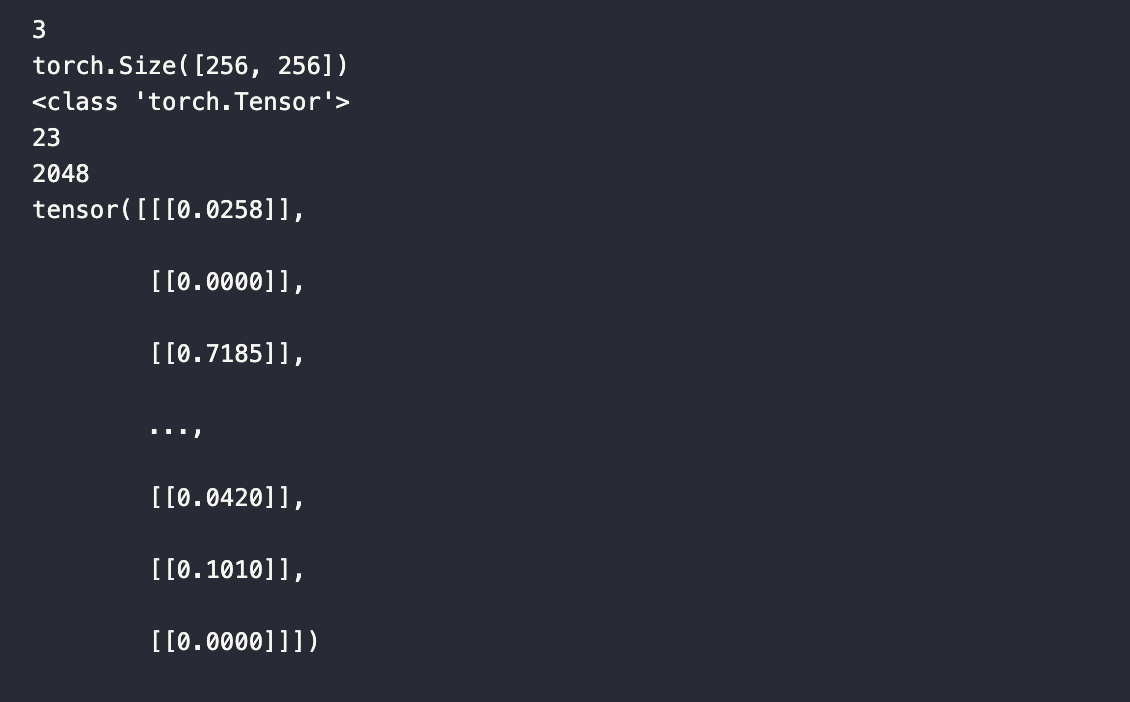
The printed data looks like the image shown below. Each data batch has a size of 128 until the end, with each entry being of size 3x256x256. The output is a PyTorch Tensor of length 128, with each entry in the output being of length 2048. The printed tensor is the output from the first entry in the data batch.
Storing your image data into a vector database
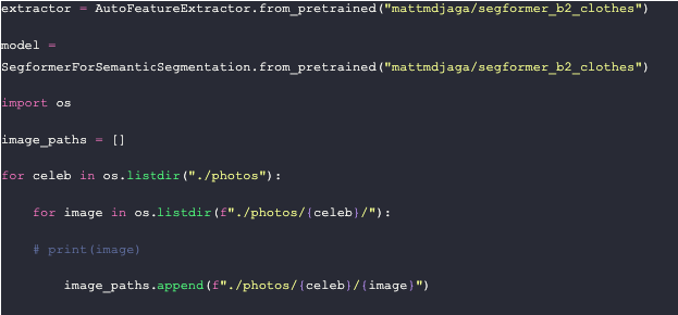
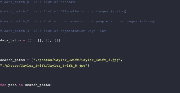
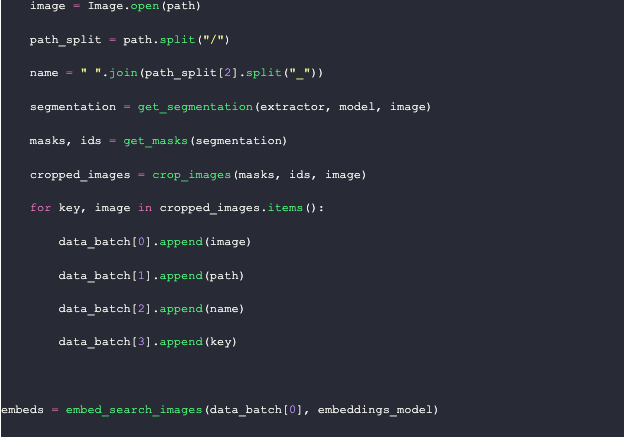
Remember that extractor and segmentation model we talked about earlier? This is where we use them. We use this pre-trained segformer model from Hugging Face. After loading the models, we put all the file paths into a list to loop through.
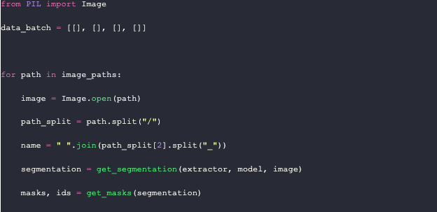
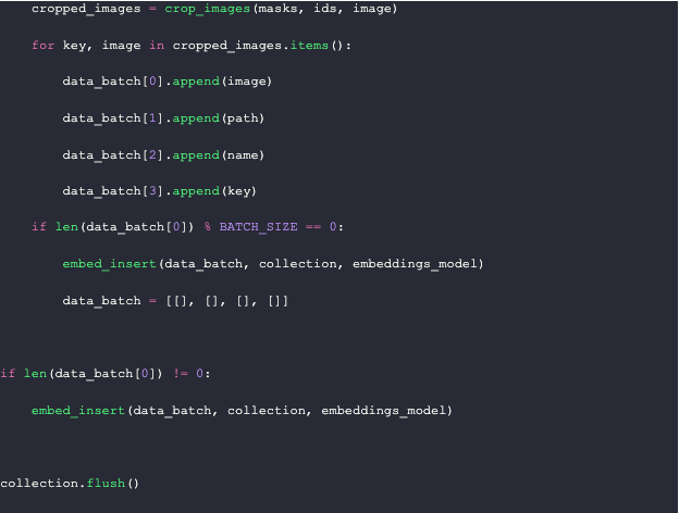
Milvus expects a list of lists as input. In this example, we use a list of 4 lists, which correspond to the image, the file path, the name, and the segmentation ID. In the `embed_insert` function, we convert the image into a vector embedding. We then loop through each file path to the images, gather their segmentation masks, and crop them. Finally, we add the images with their metadata to the data batch.
Every 128 images, we embed and insert them into Milvus, and then clear out the data batch. At the end of the loop, we embed and insert the rest of the data batch into Milvus and flush it to complete the indexing. On an M1 2021 Mac with 16GB of RAM, this process takes approximately 8 minutes to run.
Find out which celebrities you dress most like
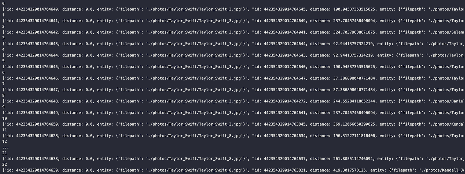
There’s a lot you can do with this setup. I will provide additional methods for matching and evaluating your fashion choices in an upcoming piece. In this example, we’ll get the top three pictures based on each segmented article of clothing. We use a couple of examples of Taylor Swift and get a perfect recall.
Generating embeddings for your input images
Similar to how we load images into the database, we need to process input images. The function for embedding search images takes two parameters: data and the (embedding) model. We use the model to get the embeddings, flatten or squeeze them depending on the number of images queried, convert them into a list, and return them.
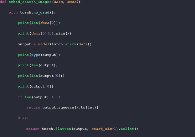
Similar to the `embed_insert` function, I added several print statements here to keep track of the data. As shown below, the `data` passed into this function is essentially the `data[0]` object, in comparison to the `embed_insert` function.
To query the database, we only need the vector embeddings, which we can obtain in a similar manner to when we added images to Milvus. However, it is useful to keep these other variables in memory to facilitate comparisons later.
Querying the vector database
Now that we have the embeddings, we can query the database. For fun, I'm adding the `time` module to track how long these queries take. In this example, we measure the query time for 23 2048-dimensional vectors. To query Milvus, we simply use the `search` function with the embeddings generated above.
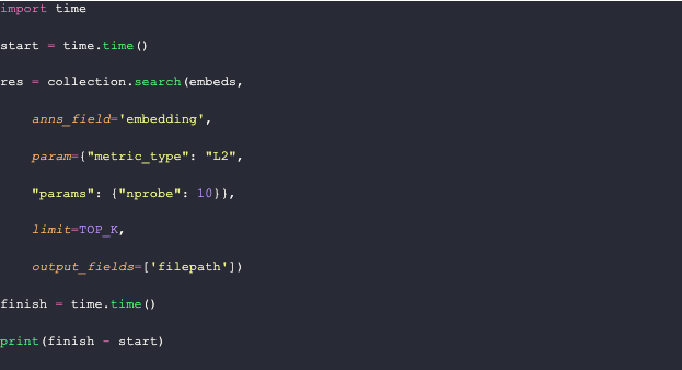
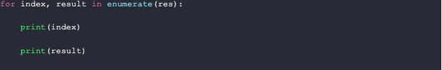
After looping through the results, we can see the generated response, shown in the image below the code.
Summary
That's all for this section. You're now ready to compare any images of yourself or your friends (with permission!) to some celebrities, including Taylor Swift, Drake, and Andre 3000. To do this, start by getting a segmentation of the clothing articles in the image using a model found on Hugging Face.
With the segmentations in hand, grab each unique segmentation from the image and crop them into separate images. Before putting these cropped images into the vector database, resize them and turn them into tensors. Then, pass them through a ResNet50 embeddings model from Nvidia to get the vector embeddings to store.
For querying, perform a similar procedure to loading the vectors. In this example, we only went as far as getting the query results. To go further, save the bounding boxes or masks in the vector database and bring them out to show specific matches. Alternatively, run the input images through the model again and do the same thing. Since we do everything locally, we can use local memory.
I hope you enjoyed this. Feel free to connect with me and share your feedback. Also, please let me know which celebrity you dress the most like!


AI accelerator insider insider
Thank you for subscribing
Level up your ai accelerator insider career & network with ai accelerator insider experts.
An email has been successfully sent to confirm your subscription.
 Follow us on LinkedIn

