
What is K-means clustering?
K-means clustering is an unsupervised machine learning algorithm used for clustering or grouping similar data points together in a dataset. It’s a partitioning algorithm that divides the data into non-overlapping clusters, where each data point belongs to a single cluster.
K-means clustering aims to minimize the sum of squared distances between each data point and its assigned centroid.
Before you dive in, can you spare a few minutes to share your expertise in generative AI and help shape the industry?
Theory — How does it work?
Step 1. First, we need to decide the value of K, which is the number of clusters we want to create. The value of K can be decided either randomly or by using some method like Elbow or Silhouette.
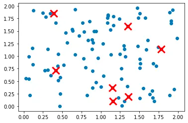
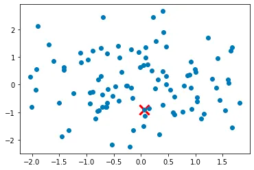
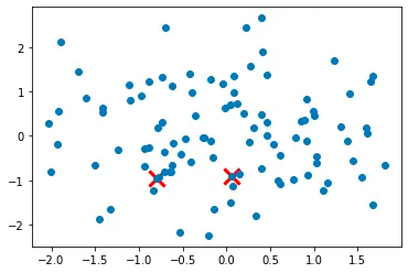
Step 2. Next, we randomly select K points from the dataset to act as initial centroids for each cluster.
Step 3. We then calculate the Euclidean distance between each data point and the centroids and assign the data point to the nearest centroid, creating K clusters.
Step 4. After assigning all data points to their nearest centroid, we update each centroid’s location by computing the mean of all the data points assigned to that centroid.
Step 5. We repeat steps 3 and 4 until the algorithm converges, which means that the centroids no longer move or the improvement in the sum of squared distances between data points and their assigned centroid becomes insignificant.
How does the code work?
Import the necessary libraries:
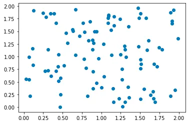
Generate or load your data into a numpy array:
Choose the number of clusters, K, and initialize the centroids randomly:
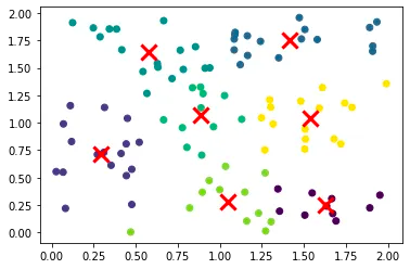
So, here we can see that data have been clustered successfully.
Limitations of K means algorithm
- K means clustering is sensitive to initial centroid selection. The algorithm may converge to a suboptimal solution if the initial centroids are not selected appropriately.
- K means clustering is sensitive to outliers.
- K means clustering is sensitive to the value of K. If K is not chosen correctly, it may give suboptimal clusters.
This is a very basic explanation of K-means clustering. The original algorithm will have a more detailed implementation. This post is to help readers get started with K-means in a very easy way.
K-means++: The next-generation clustering algorithm for efficient data segmentation
What is K-means ++
K-means++ is an improvement on the standard K-means clustering algorithm. Like K-means, it is an unsupervised learning algorithm used to group similar data points together based on their similarity. The goal of K-means++ is to initialize the cluster centers in a more intelligent way than the random initialization used by K-means, which can lead to suboptimal results.
How does K-means++ work?
Here are the main steps of the K-means++ algorithm:
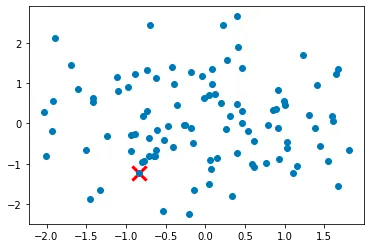
Step 1. Initialize the first cluster center by randomly selecting one data point from the dataset.
Step 2. For each data point not yet chosen as a cluster center, compute the distance between the point and the nearest cluster center.
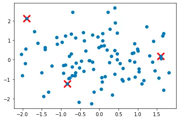
Step 3. Select the next cluster center from the remaining data points with probability proportional to the distance squared to the nearest cluster center. This ensures that the new center is far away from existing centers. This helps to ensure that the initial cluster centers are well spread out across the dataset, and not clustered in a single region.
This in turn can lead to more accurate clustering results, as the initial cluster centers can greatly influence the final clustering result.
Step 4. Repeat steps 2 and 3 until all K cluster centers have been initialized.
Proceed with the standard K-means algorithm to assign data points to clusters and update cluster centers until convergence.
By initializing the cluster centers in a more intelligent way, K-means++ is less likely to get stuck in a suboptimal solution and can lead to better clustering results.
How the code works
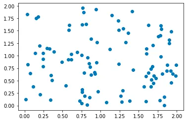
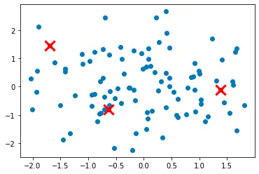
Let's create some random points and plot them:
Step 1: Initialize the first cluster center by randomly selecting one data point from the dataset.
Step 2: For each data point not yet chosen as a cluster center, compute the distance between the point and the nearest cluster center.
Step 3: Select the next cluster center from the remaining data points with probability proportional to the distance squared to the nearest cluster center.
Step 4: Repeat steps 2 and 3 until all K cluster centers have been initialized.

In this step, we repeat steps 2 and 3 until all K cluster centers have been initialized. We first set the number of clusters to k. We then initialize the first cluster center as described in step 1. We use a while loop to repeat steps 2 and 3 until len(centers) equals k.
Step 5: Proceed with the standard K-means algorithm to assign data
Cons of K-means++
While K-means++ is a popular and effective clustering algorithm, it is not without its limitations and drawbacks. Here are some of the main cons of K-means++:
- Sensitive to initial seed: Although K-means++ helps to ensure a good initial set of cluster centers, the algorithm is still sensitive to the initial seed or starting point. Different initial seeds can result in different cluster centers and ultimately different clustering results.
- Difficulty in determining optimal number of clusters: K-means++ requires the number of clusters to be specified beforehand. However, determining the optimal number of clusters is not always straightforward and can require trial and error or other methods such as the elbow method or silhouette score.
- Prone to local optima: Like traditional K-means, K-means++ is prone to getting stuck in local optima, which can result in suboptimal clustering results. This can be mitigated by running the algorithm multiple times with different initial seeds and selecting the best result.
- Assumes spherical clusters: K-means++ assumes that clusters are spherical and have a similar size and density. This may not be appropriate for datasets with non-spherical or irregularly shaped clusters.
- Can be computationally expensive: K-means++ can be computationally expensive for large datasets or high-dimensional data. The algorithm requires multiple iterations of computing distances and probabilities, which can be time-consuming for large datasets or high-dimensional data.
- Struggles with high dimensional data
Overall, K-means++ is a useful and widely used clustering algorithm, but it is important to be aware of its limitations and potential drawbacks.
When to use Kmeans++
K-means++ is a good choice when the number of clusters is known or can be estimated beforehand. It’s also a good choice when the data has a clear underlying structure and the clusters are relatively well-separated. K-means is intended to be used when all of your features are numeric.
Here are some scenarios where K-means++ can be a good choice:
- Image segmentation: K-means++ can be used for image segmentation, where the goal is to partition an image into different regions based on color or texture. In this case, the number of clusters can be estimated based on the number of distinct regions in the image.
- Market segmentation: K-means++ can be used for market segmentation, where the goal is to identify groups of customers with similar purchasing behavior or preferences. In this case, the number of clusters can be estimated based on the number of distinct customer segments.
- Inventory categorization
This is an intuition to K-means ++. The original implementation may be different from this.
Stay tuned for more such explanations.


AI accelerator insider insider
Thank you for subscribing
Level up your ai accelerator insider career & network with ai accelerator insider experts.
An email has been successfully sent to confirm your subscription.
 Follow us on LinkedIn

