
Welcome (or welcome back!) to the AI for social good series! In the second part, of this two-part series of articles, we will look at how artificial intelligence (AI) coupled with the power of open-source tools and techniques like deep learning can help us further the quest for finding extra-terrestrial intelligence!
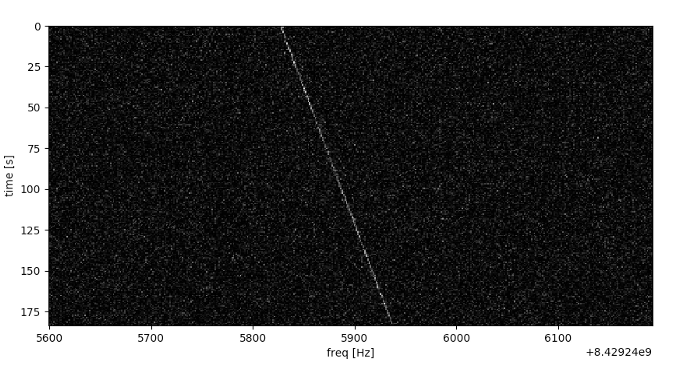
In the first part of this two-part series, we formulated our key objective and motivation behind doing this project. Briefly, we were looking at different radio-telescope signals simulated from SETI (Search for Extra-terrestrial Intelligence) Institute data. We leveraged techniques to process, analyze and visualize radio signals as spectrograms, which are basically visual representations of the raw signal.
The key focus for us in this article will be to try and build a robust radio signal classifier using deep learning for a total of seven different types of signals!
Loading SETI Signal Data
Like we discussed in the previous article, the simulated SETI radio-signal dataset is available in Kaggle. Remember, the processed dataset is available in the primary_small folder. After unzipping its contents this is how the directory structure looks like.
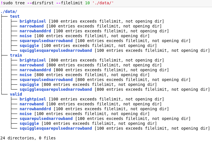
We have a total of 7 different signal classes to classify, each class has a total of 800 samples for training, 100 for validation and test respectively. Considering noise has been added to the simulated signal data coupled with the fact that we have less number of samples per class makes this a tough problem to solve! Before we get started, let’s load the necessary dependencies we will be using for building models. We will leverage the tf.keras API from TensorFlow here.
./data/train
./data/valid
./data/test
Visualize Sample SETI Signals
Just to recap from our last article and take a peek at the different types of signals we are dealing with, we can visualize their spectrograms using the following code.
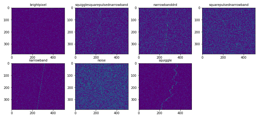
Things look to be in order with regard to the different signal samples we are dealing with!
Data Generators and Image Augmentation
Since we have a low number of training samples per class, one strategy to get more data is to generate new data using image augmentation. The idea behind image augmentation is exactly as the name sounds. We load in existing images from our training dataset and apply some image transformation operations to them, such as rotation, shearing, translation, zooming, flipping and so on, to produce new, altered versions of existing images.
Due to these random transformations, we don’t get the same images each time. We need to be careful with augmentation operations though based on the problem we are solving so that we don’t end up distorting the source images too much.
We will be applying some basic transformations to all our training data but keep our validation and test dataset as it is except just scaling the data. Let’s build our data generators now.
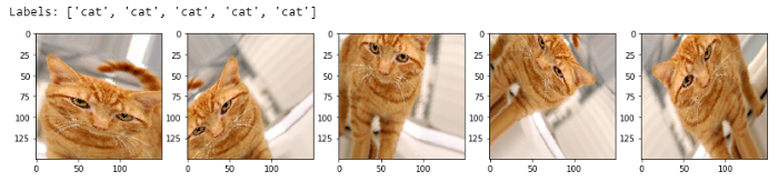
We can now build a sample data generator just to get an idea of how the data generator coupled with image augmentation works.
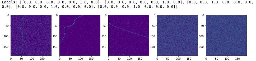
The labels are one-hot encoded given that we have a total of 7 classes so each label is a one-hot encoded vector of size 7.
Deep Transfer Learning with CNNs
The idea of transfer learning is not a new concept and is something which is very useful when we are working with less data. Given that we have a pre-trained model, which was trained previously on a lot of data, we can use this model on a new problem with less data and should ideally get a model which performs better and converges faster.
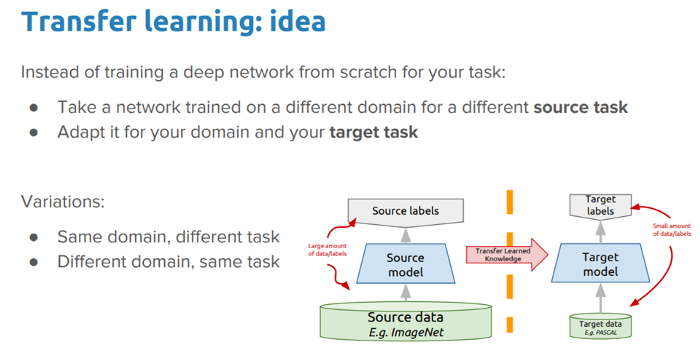
There are a wide variety of pre-trained CNN models which have been trained on the ImageNet dataset having a lot of images belonging to a total of 1000 classes. The idea is that these models should act as effective feature extractors for images and can also be fine-tuned to the specific task we perform. Pre-trained models can be frozen completely where we don’t change the layer weights at all when we train on the new dataset or we can fine-tune (partially or completely) the model weights as we train on the new dataset.
In our scenario, we will try out partial and complete fine-tuning of our pre-trained models.
Pre-trained CNN Models
One of the fundamental requirements for transfer learning is the presence of models that perform well on source tasks. Luckily, the deep learning world believes in sharing. Many of the state-of-the art deep learning architectures have been openly shared by their respective teams. Pre-trained models are usually shared in the form of the millions of parameters/weights the model achieved while being trained to a stable state. Pre-trained models are available for everyone to use through different means.
Pre-trained models are available in TensorFlow which you can access easily using its API. We will be showing how to do that in this article. You can also access pre-trained models from the web since most of them have been open-sourced.
For computer vision, you can leverage some popular models including,
The models we will be using in our article will be VGG-19 and ResNet-50.
VGG-19 model
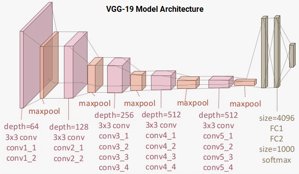
The VGG-19 model is a 19-layer (convolution and fully connected) deep learning network built on the ImageNet database, which is built for the purpose of image recognition and classification. This model was built by Karen Simonyan and Andrew Zisserman and is mentioned in their paper titled ‘Very Deep Convolutional Networks for Large-Scale Image Recognition’. I recommend all interested readers to go and read up on the excellent literature in this paper. The architecture of the VGG-19 model is depicted in the following figure.
ResNet-50 model
The ResNet-50 model is a 50-convolutional block (several layers in each block) deep learning network built on the ImageNet database. This model has over 175+ layers in total and is a very deep network. ResNet stands for Residual Networks. The following figure shows the typical architecture of ResNet-34.
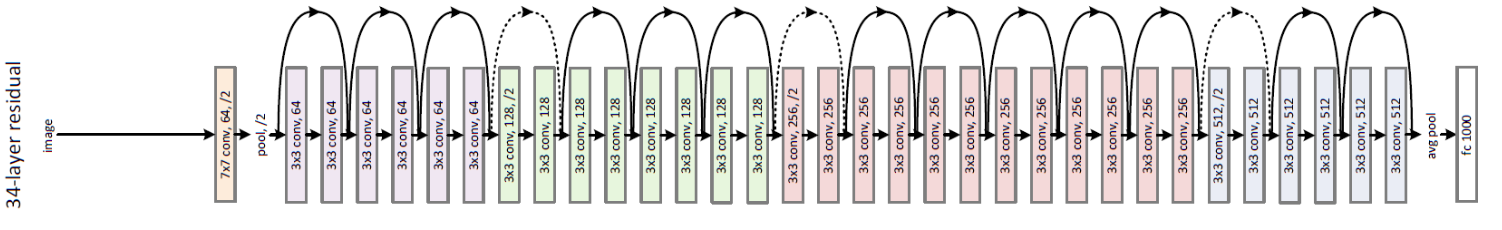
In general, deep convolutional neural networks have led to major breakthroughs in image classification accuracy. However, as we go deeper; the training of neural network becomes difficult. The reason for this often is because of the vanishing gradient problem . Basially as the gradient is back-propagated to the shallower layers (closer to the input), repeated tensor operations make the gradient really small. Hence, the accuracy starts saturating and then degrades also. Residual Learning tries to solve these problems with residual blocks.
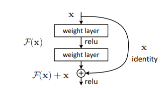
Leveraging skip connections, we can allow the network to learn the identity function (depicted in the above figure), which allows the network to pass the input through the residual block without passing through the other weight layers. This helps in tackling the problems of vanishing gradients and also keeping a focus on the high-level features which sometimes get lost with multiple levels of max-pooling.
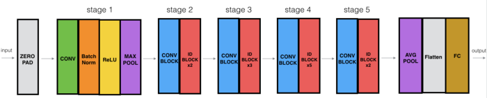
The ResNet-50 model which we will be using, consists of 5 stages, each with a Convolution and Identity block. Each convolution block has 3 convolution layers and each identity block also has 3 convolution layers.
Deep Transfer Learning with VGG-19
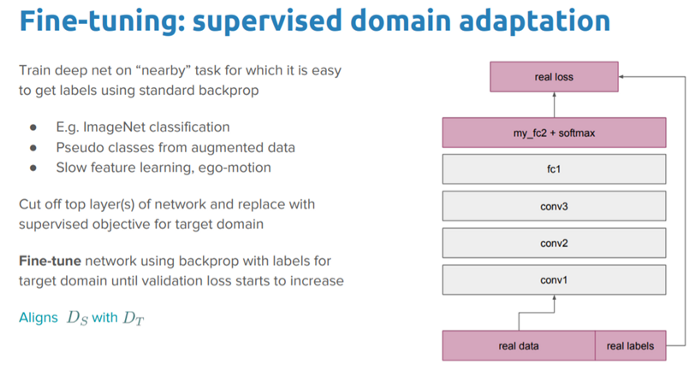
The focus here will be to take the pre-trained VGG-19 model and then perform both partial and complete fine-tuning of all the layers in the network. We will add the regular dense and output layers in the model for our downstream classification task.
Partial Fine-tuning
We will start our model training by taking the VGG-19 model and fine-tune the last two blocks of the model. The first task here is the build the model architecture and also specify which blocks \ layers we want to fine-tune.
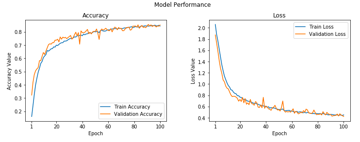
Now we will train the model for 100 epochs. I save the model after each epoch because I have a lot of space. I wouldn’t recommend to do this practically unless you have a lot of storage. You can always leverage a callback like ModelCheckpoint to focus on storing only the best model.
We can view the overall model learning curves using the following code snippet.
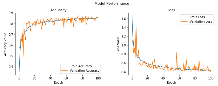
Looks decent but definitely a lot of fluctuations with regard to the loss and accuracy over time for the validation dataset.
Complete Fine-tuning
For our next training process, we will take the VGG-19 model and fine-tune all the blocks and add in our own dense and output layers.
The learning curves for the training process are depicted in the following figure.
Looks to be more stable as the epochs increase with regard to the validation accuracy and loss.
Deep Transfer Learning with ResNet-50
The focus in this section will be taking the pre-trained ResNet-50 model and then perform complete fine-tuning of all the layers in the network. We will add the regular dense and output layers as usual.
Complete Fine-tuning
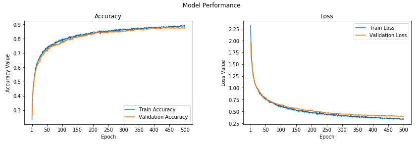
For our training process, we will load the pre-trained ResNet-50 model and fine-tune the entire network for 500 epochs. Let’s start by building the model architecture.
Let’s now train the model for a total of 500 epochs.
The learning curves for our trained model can be observed in the following figure.
Evaluating Model Performance on Test Data
It is now time to put our trained models to the test. We will do so by making predictions on the test dataset and evaluating model performance based on relevant classification metrics for our multi-class classification problem.
Load Test Dataset
We start by loading out test dataset and labels leveraging our data generator we had built previously.
Found 700 images belonging to 7 classes.
((700, 192, 192, 3), (700,))
Build Model Performance Evaluation Function
We will now build a basic classification model performance evaluation function, which we will use to test the performance of each of our three models.
We are now ready to test our models’ performance on the test dataset
Model 1 — Partial fine-tuned VGG-19
Here we evaluate the performance of our partially fine-tuned VGG-19 model on the test dataset.
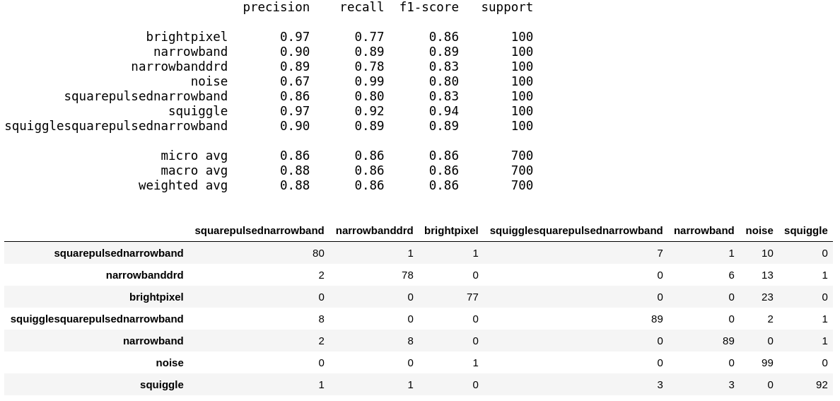
An overall accuracy \ f1-score of 86% on the test dataset which is pretty decent!
Model 2 — Complete fine-tuned VGG-19
Here we evaluate the performance of our completely fine-tuned VGG-19 model on the test dataset.
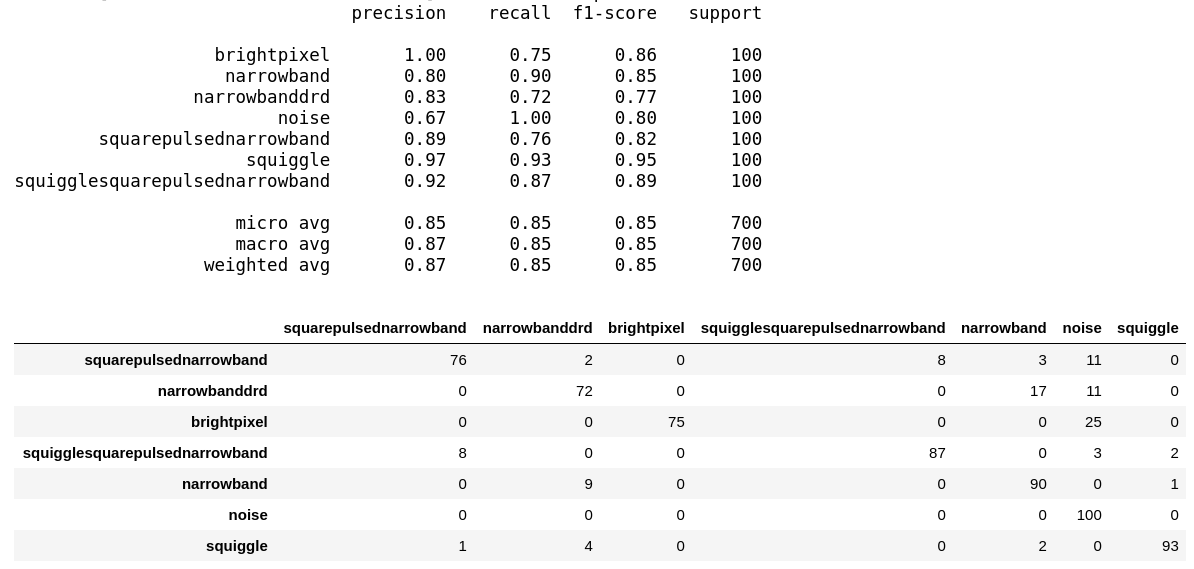
An overall accuracy \ f1-score of 85% on the test dataset which is slightly lesser than the partially fine-tuned model.
Model 3 — Complete fine-tuned ResNet-50
Here we evaluate the performance of our completely fine-tuned ResNet-50 model on the test dataset.
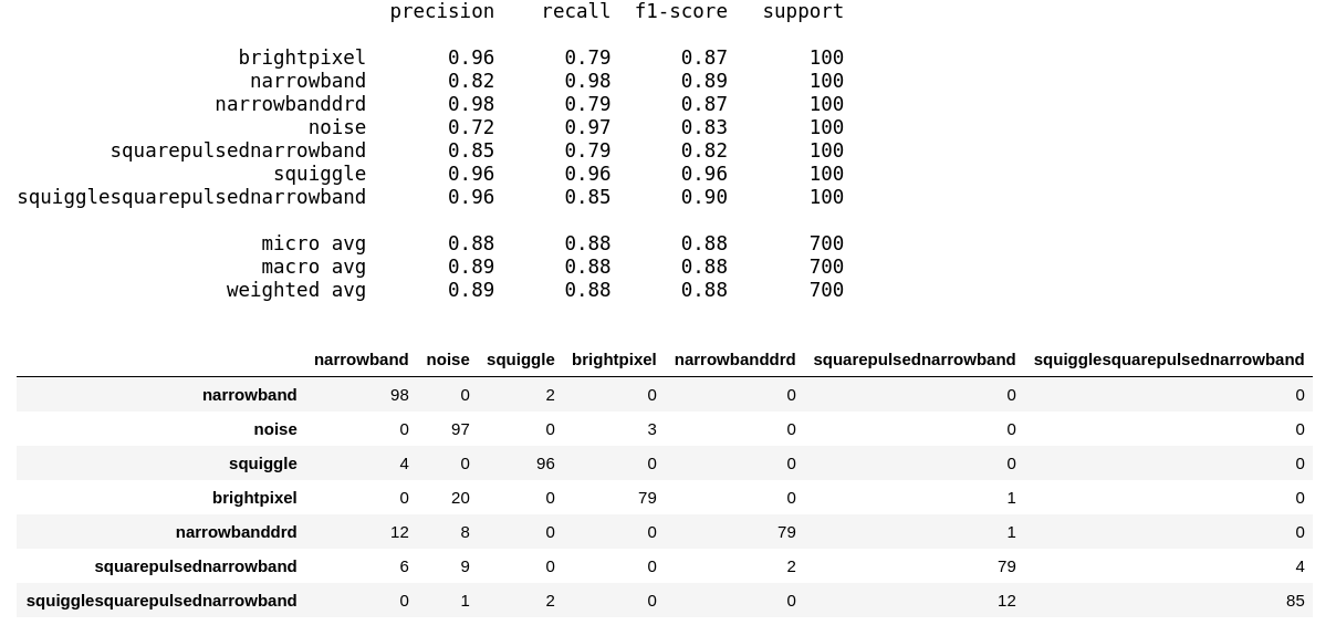
We get an overall accuracy \ f1-score of 88% which is definitely the best model performance yet on the test dataset! Looks like the ResNet-50 model performed the best, given the fact that we did train it for 500 epochs.
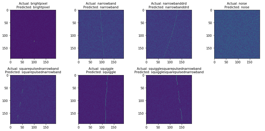
Best Model Predictions on Sample Test Data
We can now use our best model to make predictions on sample radio-signal spectrograms.
Conclusion
This brings us to the end of our two-part series on leveraging deep learning to further the search of extra-terrestrial intelligence. You saw how we converted radio-signal data into spectrograms and then leveraged the power of transfer learning to build classifiers which performed pretty well even will really low number of training data samples per class.


AI accelerator insider insider
Thank you for subscribing
Level up your ai accelerator insider career & network with ai accelerator insider experts.
An email has been successfully sent to confirm your subscription.
 Follow us on LinkedIn

