In this two-part series of articles, we will look at how Artificial intelligence (AI) coupled with the power of open-source tools and frameworks can be used to solve a very interesting problem in a non-conventional domain — the quest for finding extra-terrestrial intelligence!

Perhaps many of you are already familiar with the SETI (Search for Extra-terrestrial Intelligence) Institute, which focuses on trying to find out the existence of extra-terrestrial intelligence out in the universe and as its mission suggests, “exploring, understanding and explaining the origin and nature of life in the universe and the evolution of intelligence”. Recently, I had come across an open dataset from SETI on Kaggle which talks about SETI focusing on several public initiatives tied around leveraging AI on their datasets in the form of competitions which had occurred in the past. While the competition is inactive now, a subset of this data is still available for analysis and modeling which is the main focus of our articles in this series.

We will be looking at analyzing data sourced by SETI as a part of their past initiative, ML4SETI — Machine Learning 4 the Search for Extra Terrestrial Intelligence. This data for this initiative is simulation data based on radio signals The goal here was for data scientists to find a robust signal classification algorithm for use in the mission to find E.T. radio communication. The key focus here being able to classify different types \ classes of signals accurately.

Motivation & Significance

The SETI Institute is dedicatedly researching and working on methods to improve their search for extra-terrestrial intelligence. One of their key instruments accelerating this search is known as the Allen Telescope Array (ATA), which is situated at the Hat Creek Observatory, located in the Cascade Mountains just north of Lassen Peak, in California.

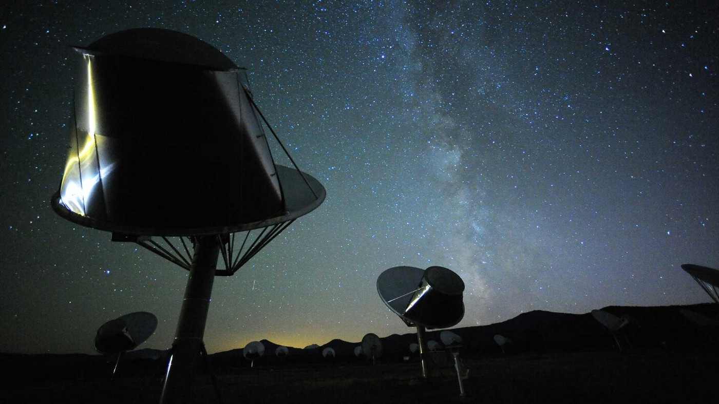
The Allen Telescope Array helps in radio-signal based searches and is speeding up SETI targeted searching by a factor of at least 100. The motivation for applying AI or Deep Learning here can be maifold.

• Deep Learning Models optimized to distinguish between different signals may decrease search time
• Efficiency and maybe even new and better ways to find out extra-terrestrial intelligence as they observe signals from star systems

While the data we will be using here is simulation data based on radio signals, they are very much in line with the real data captured by radio-telescopic devices at SETI. We will take a brief look at this now.

Understanding SETI Data

The information presented here was based on insights which I gathered from researching on details about SETI data when they had this competition in collaboration with IBM a while back. Details of the challenge are presented here for folks who might be interested and a lot of the background information about the setup and data are mentioned in this useful article.

Allen Telescope Array Architecture

The Allen Telescope Array (ATA) consists of several relatively small dishes (antennas) extending over about 1 km. This provides a very high quality beam shape (the spot in the sky to which the telescope is most sensitive). The ATA is actually optimized to cover frequencies between 1000 MHz — 15000 MHz. The ATA combines the signals from different dishes, using a process called “beamforming”. Typically using this process, the ATA observes radio signals from very small windows of the sky about specific stellar systems. On a high level, the ATA has four main conceptual systems as explained in the official page.

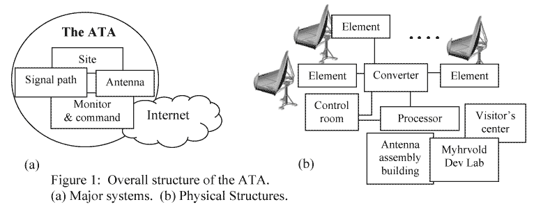
• The antenna collects the radiation from space;
• The signal path brings the radiation from the feed (which is located at the antenna focus) back to the user
• The monitor and command systems allow the dishes to be accurately moved, and the signal path controlled
• The site includes the overall antenna configuration, as well as other infrastructure.

The ATA will permit remote users to access and use the instrument via a secure Internet connection.

Radio-Telescope Time Series Signals

From a usage perspective, three separate beams may be observed simultaneously and are used together to make decisions about the likelihood of observing intelligent signals.

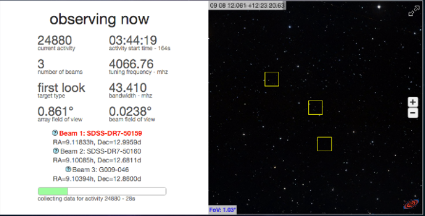
The software that controls the data acquisition system, analyzes this radio signal time-series data in real-time and writes data out to disk. It is called SonATA (SETI on the ATA).

To find relevant signals, the SonATA software calculates the signal power as a function of both frequency and time, and focuses on signals with power greater than the average noise power that persist for more than a few seconds. The best way of representation of the power as a function of frequency and time is through spectrograms, or “waterfall plots”.

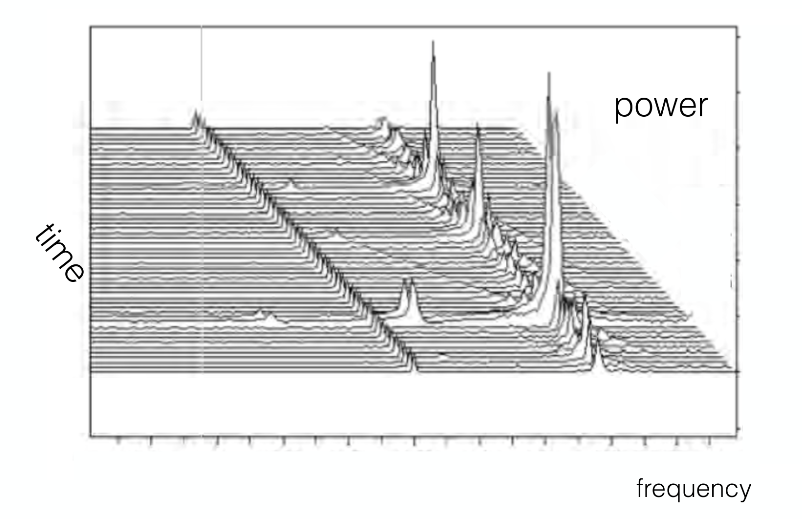
A sample spectrogram of real radio-signal data from the ATA is depicted in the following figure. This is a classic example of what is called as a “narrowband” signal, which is what SonATA primarily searches for in the data.

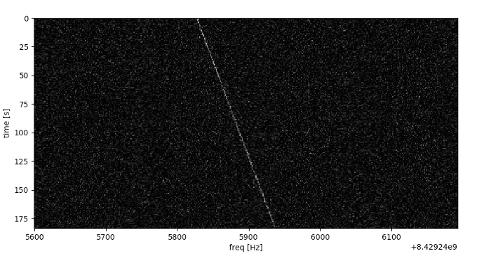
The power of the signal is represented on a black & white scale. We have time on the y-axis and frequency (Hz) on the x-axis. You can clearly see a signal starting at approximately 8429245830 Hz and drifting up to 8429245940 Hz over the 175 second observation.

The Need for Analyzing Radio-Signal Data

The reason SETI is capturing this data and searching for specific patterns in the signals is because this is the kind of signal we use to communicate with our satellites in space. Hence there is a hope that a seemingly advanced extra-terrestrial (E.T.) civilization might transmit a signal to us if they were trying to get our attention!

Getting Simulated SETI Data

Now that we have enough background information on SETI and its data. Let’s try and get the dataset which we will be using to train our deep learning models. The competition ML4SETI is long over unfortunately but fortunately for us, a subset of the data is still available. Feel free to check out the ML4SETI ‘Getting Started’ page to get an idea of how to get the dataset. If you feel like diving right into the data without reading the background information, just head over to this Jupyter Notebook! An easier way to get this dataset is from Kaggle.

Since there were challenges of working with real data, a set of simulated signals were built to approximate this real signal data. Typically there are a number of signal classes that SETI Institute researchers often observe. For the purpose of this dataset there were a total of seven different classes.

• brightpixel
• narrowband
• narrowbanddrd
• noise
• squarepulsednarrowband
• squiggle
• squigglesquarepulsednarrowband

The class names are basically descriptive how they look like in spectrograms.

Main Objective

It is easy to define our main objective now that we have all our background information and our data. Give a total of seven different radio-signal classes including noise and a total of 1000 samples per class, leverage deep learning models to build an accurate classifier. While we will be building the deep learning models in the second part of this series, in the remaining sections of this article, we will be diving deeper into the dataset to gain a better understanding of what we are dealing with.

Analyzing Simulated SETI Data

We used the small version of the SETI data primary_small_v3 in its raw format just to show how to load and process the data. Remember to process the signal data you will be needing the open-source ibmseti package. You can install it using pip install ibmseti. Let’s load up the raw dataset now before some basic processing and analysis.

7000

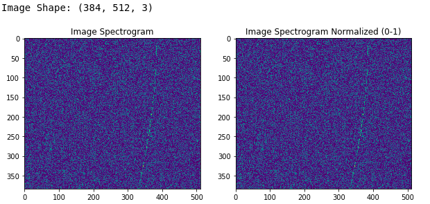
This tells us we have a total of 7000 signal samples in our dataset. Let’s try processing and visualizing one of these signals.

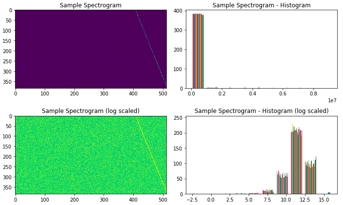
Thus based on the visuals above, we have successfully processed a narrowband signal into a spectrogram before visualizing it. Let’s look at the total number of signal samples per-class.

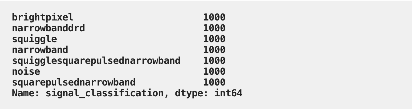
Like we mentioned before, we have a total of 1000 samples per class, which is frankly not a lot! More on that later. Let’s process and visualize some sample signals with spectrograms.

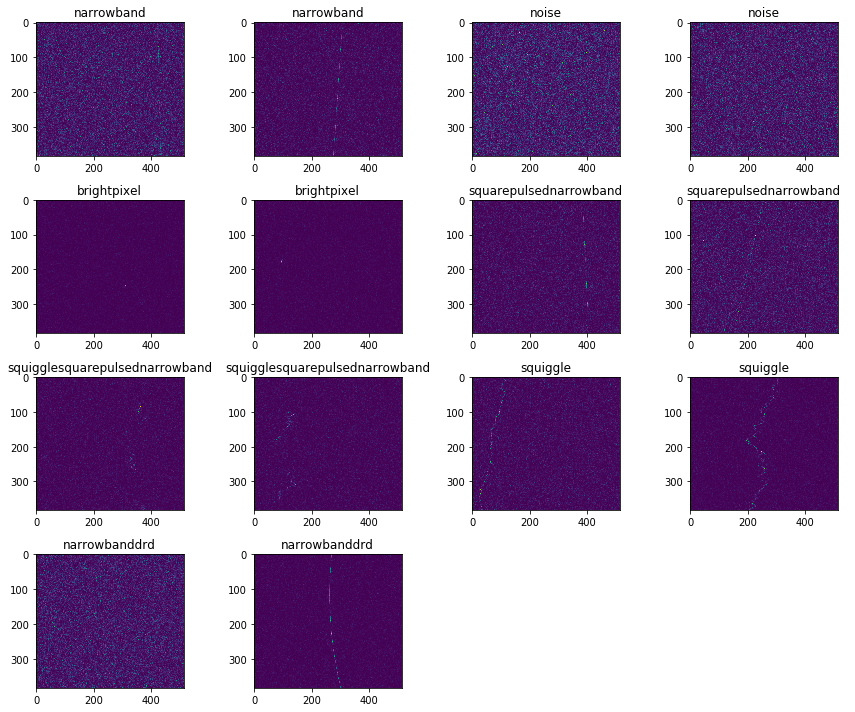
This kind of gives us an idea of how the different signals look like. You can see that these signals are not always very distinguishable and hence makes this a tougher classification challenge.

Loading Processed SETI Data

Now, for the remainder of this article and the next one in this series, you can manually leverage the ibmseti package and process each signal into a spectrogram or just download and use the already processed spectrogram files from the dataset available in Kaggle. Remember, the processed dataset is available in the primary_small folder. After unzipping its contents this is how the directory structure looks like.

We have a total of 7 classes and 800 training samples, 100 validation samples and 100 test samples per class. Let’s look at some sample processed spectrogram signal files now.

Loading and Visualizing Spectrograms with Keras

The Keras framework has some excellent utilities to work with image files containing these spectrograms. Following snippet showcases this on a sample spectrogram.

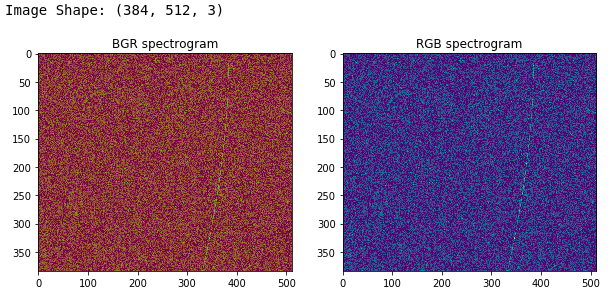
Loading and Visualizing Spectrograms with OpenCV

There are a lot of OpenCV fans out there who love using the framework for all their image processing needs. You can use that too for working with spectrograms. Do remember that OpenCV loads these images by default in the BGR format and not RGB. We showcase the same in the following code.

Visualizing Processed SETI Sample Data

Let’s now visualize the seven different sample signals which we selected from the processed dataset we will be using later for classification.

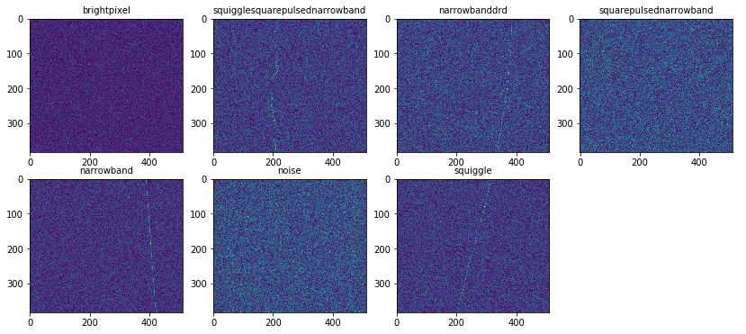
This shows us the different types of radio-signals in our dataset which are processed and ready to be used.

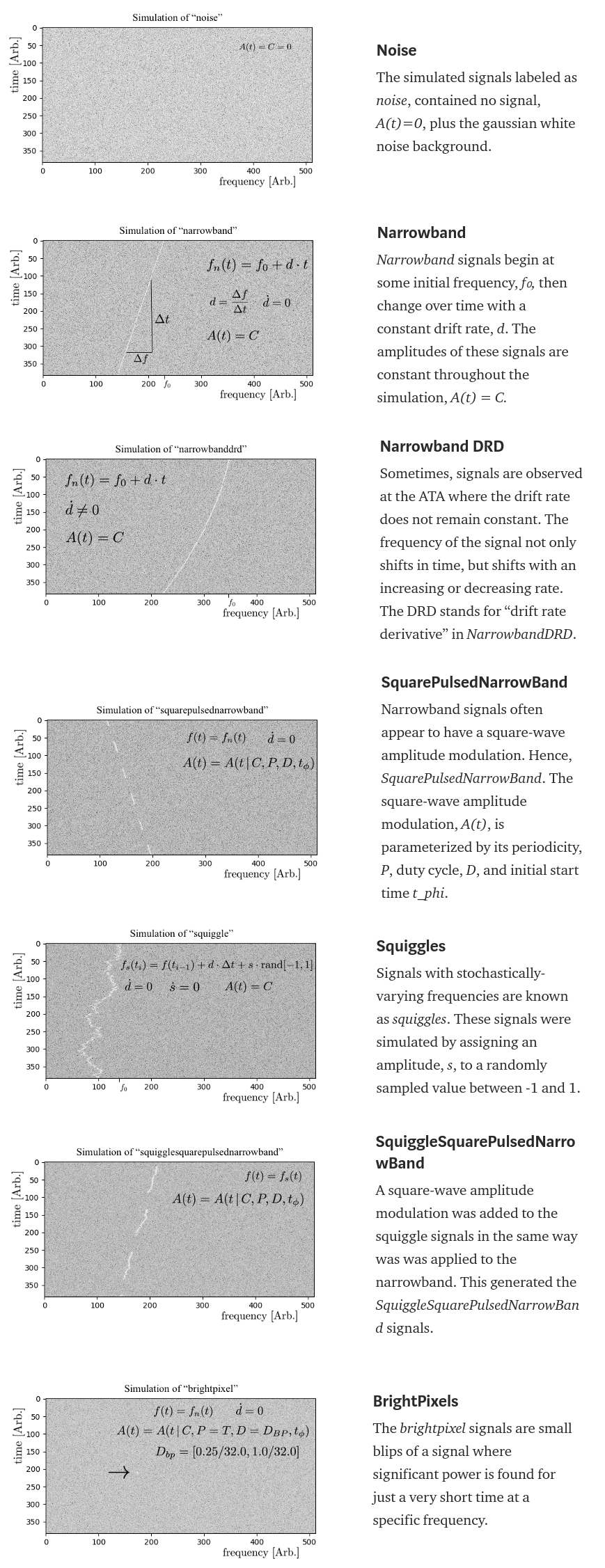
Understanding the Radio-Signal Simulation Data

All simulation signals here were generated by a sum of the signal and a noise background. The following background information about signals, has been collated from this wonderful article to understand about each signal in more detail

Deep Learning on SETI Data

Given that we have spectrogram images for our seven signal classes, we can leverage vision-based deep learning models to build robust image classifiers. In the next article in this series, we will be leveraging convolutional neural networks to see how we can build accurate classifiers to distinguish between these signal classes!

Brief on Convolutional Neural Networks

The most popular deep learning models leveraged for computer vision problems are convolutional neural networks (CNNs)!

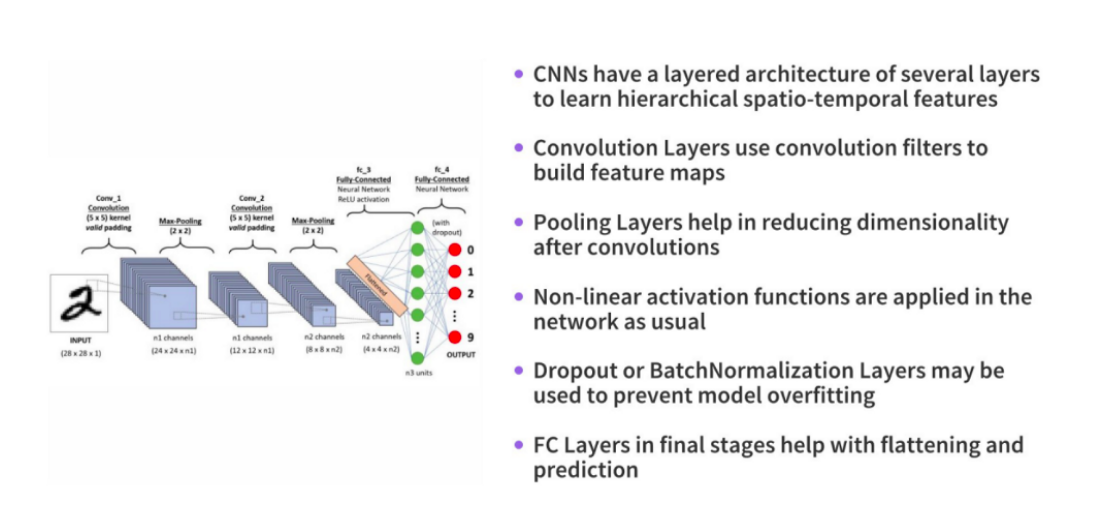
CNNs typically consist of multiple convolution and pooling layers which help the deep learning model in automatically extracting relevant features from visual data like images. Due to this multi-layered architecture, CNNs learn a robust hierarchy of features, which are spatial, rotation, and translation invariant.

The key operations in a CNN model are depicted in the figure above. Any image can be represented as a tensor of pixel values. The convolution layers help in extracting features from this image (forms feature maps). Shallower layers (closer to the input data) in the network learn very generic features like edges, corners and so on. Deeper layers in the network (closer to the output layer) learn very specific features pertaining to the input image. The following graphic helps summarize the key aspects of any CNN model.

We will be leveraging the power of transfer learning, where we use pre-trained deep learning models (which have already been trained on a lot of data). More on that in the next article!

Next Steps

In the next article we will build deep learning classifiers based on CNNs to classify SETI signals accurately. Stay tuned!